SMS:Animations
At a glance
- Several types of AVI animations (film loops) can be generated by SMS
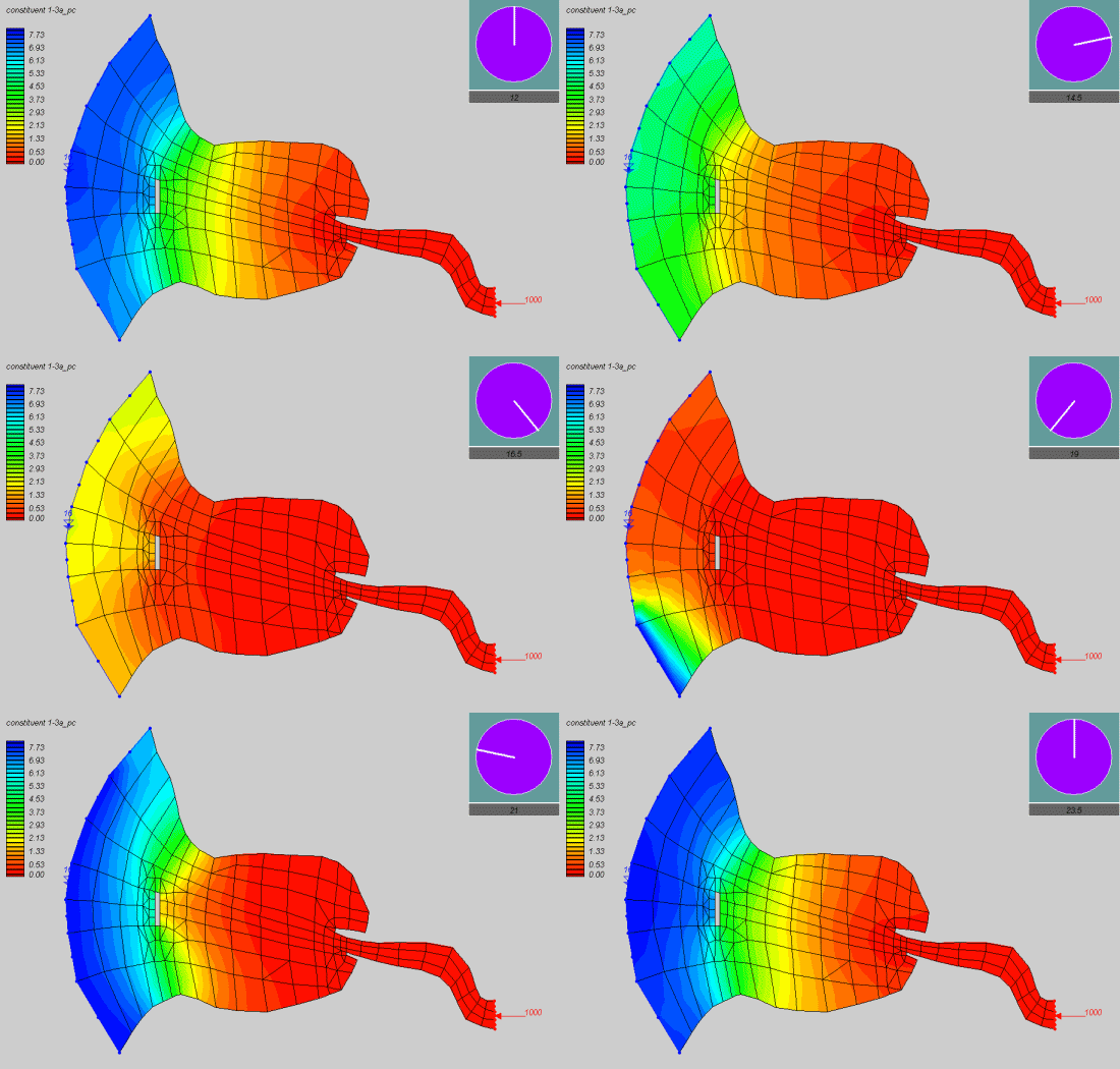
- Transient data animation shows model changes through time (contours, vectors, etc.)
- Flow trace uses vector data to generate flow paths through the geometry
- Drogue plots use user specified starting locations and show how the particles would flow through a vector field
- Multiple view animations show the data while transitioning between different views
- Plot window animations show plots changing through time
Animations in SMS provide a powerful tool for visualizing solution data.
Film Loop Setup Wizard
To create an animation select Data | Film Loop to open the Film Loop Setup wizard. The pages in the Film Loop Setup wizard include:
- General Options
- Display Options
- Time Step Options
- Multiple Views
- Drogue Plot Options
- Flow Trace Options
Animation Types
Flow Trace Animations
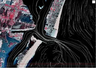
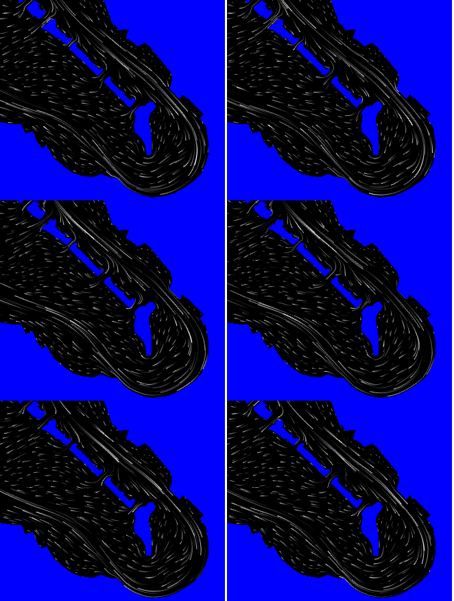
Flow trace animation is a technique used to visualize vector fields in SMS. It can be thought of as dropping tiny drops of dye into a fluid field in a random distribution and watching the flow pattern created. The process can also be thought of as creating particles of zero mass, and letting the vectors in the vector field be forces pushing the particles around. The Flow Trace portion of the Film Loop Setup dialog allows controlling the flow trace. This entire portion of the dialog is disabled if no vector data exists for the current data set. The top radio group specifies whether the flow trace should be created for a steady state or dynamic system. Below this, specify the density of particles or dye droplets by specifying the average number of particles for each cell or element. The number of frames required for a droplet to become dispersed is represented as a portion of the animation in the Decay ratio field.
The path of each particle is defined by tracing the particle. A starting position is defined randomly in the mesh or grid. Successive particle locations are computed by applying the forces of the vector field to the current location. At the new point, the velocity and direction are sampled. If the particle has traveled farther than the Flow trace length limit, or the velocity has changed more than the Velocity difference limit, the step is broken into two steps of half the step size. This process is repeated, until a sequence of valid points within the limits are defined for each frame. Therefore, the smaller the values of the Flow trace length limit and Velocity difference limit, the more precisely the particles will imitate the vector field. Generally, the default values are sufficient.
The Average particle speed is used to scale the vector field, thus changing the distance each particle or droplet travels. This is useful for vector fields with extreme magnitudes. For a low magnitude data set, the particles may not move very far. While this sluggish motion is accurate for the data, scaling the vector field up, and exaggerating the motion causes the flow patterns to be more visible. Similarly, in high magnitude fields the particles may become long streaks and scaling the values down may result in a clearer picture of the flow patterns.
Transient Data Animations
Animation Clock
Since animations are simulating the passage of time, it is natural to display a clock, which indicates the time reference for each frame of the animation. The Display Clock toggle controls whether a clock will be displayed. The Options button brings up the Legend Options dialog with a control to specify a digital clock face or analog.
Animation Time Control
Animation can be applied to any object with a dynamic dataset. Start by defining the beginning and ending time for the animation sequence and the time step between subsequent frames. As each frame is generated, data values corresponding to the current time are loaded into memory and the image is redrawn using the current display options. The display options may be modified while setting up an animation using the display options button in the Display Options portion of the dialog.
The strip in the center of the Data Options portion of the Film Loop Setup dialog displays the allowable time values for the current data function(s) and the selected range to be animated. Select a time range to animate graphically on this scale, or explicitly in the edit fields below the time step strip. The legal time range displayed in the strip is based on the current scalar and vector data set(s). SMS allows animation of only scalar or vector data while the other remains constant. This normally is only used when a static field such as elevation is displayed with a varying velocity field or a static velocity field is displayed over a changing scalar field such as constituent dispersion or sediment deposition.
The total number of frames generated in the film loop can be defined by either matching the time steps (one frame per time step) or by using a constant interval (e.g., one frame for every two-hour interval). If the Match Time Steps option is chosen, extra frames can be created between each time step using linear interpolation of the data values at the specified time steps.
Animation Playback
Once a new animation has been generated, SMS launches the AVI player and plays the animation. The speed of playback can be adjusted using the Speed scroll bar. The maximum speed depends on the speed of the computer and the size of the image being animated. The smaller the image, the faster the maximum playback speed.
Related Topics
SMS – Surface-water Modeling System | ||
|---|---|---|
| Modules: | 1D Grid • Cartesian Grid • Curvilinear Grid • GIS • Map • Mesh • Particle • Quadtree • Raster • Scatter • UGrid |  |
| General Models: | 3D Structure • FVCOM • Generic • PTM | |
| Coastal Models: | ADCIRC • BOUSS-2D • CGWAVE • CMS-Flow • CMS-Wave • GenCade • STWAVE • WAM | |
| Riverine/Estuarine Models: | AdH • HEC-RAS • HYDRO AS-2D • RMA2 • RMA4 • SRH-2D • TUFLOW • TUFLOW FV | |
| Aquaveo • SMS Tutorials • SMS Workflows | ||


