User talk:Mburton
13.3 Coverages Tools
This article describes tools from the SMS toolbox designed to perform specialized modifications to to feature objects inside coverages.
Coverages Tools
Template:Contours from Raster Elevation
Features from Raster
The Features from Raster tool derives features such as streams and roadway embankments from an elevation raster.
Input Parameters
- Input raster – Select the input elevation raster.
- Feature type – Select the feature type to generate.
- "Stream" – This option generates stream lines given the threshold area for stream generation.
- "Ridge" – This option generates ridge lines for the inverted raster given the threshold area for ridge generation.
- Threshold area – The threshold area to use for stream or ridge generation.
- Pre-processing engine – Which pre-processing engine to use.
- "rho8" – Computes flow directions and accumulations using the Rho8 algorithm.
- "Whitebox full workflow" – Computes flow directions and accumulations using the Whitebox tool full workflow algorithm that uses a standard D8 method for computing flow directions.
Output Parameters
- Output coverage – Defines the name of the tool-generated output coverage
- Breached, Flow direction, and Flow accumulation rasters are also generated from this tool. The names of these are currently hardwired to the original raster names ending in _breached, _flowdir, and _flowaccum respectively. An additional extension is added to the end of the raster name based on the pre-processing engine used.
Current Location in toolbox
Coverages/Features from Raster
Polygon from Raster Bounds
The Polygon from Raster Bounds tool creates a new coverage with polygons bounding all of the active regions of the raster. Any inactive regions that fall within an interior polygon will be deleted automatically.
Inactive regions of a raster are determined by the NODATA value of the raster.


Input Parameters
- Input raster – The raster for which the active boundary polygon will be created.
Output Parameters
- Output coverage – The new coverage to be created, containing the boundary polygon for the active region of the input raster.
Current Location in Toolbox
Coverages/Polygon from Raster Bounds
Polygons from Arcs
The Polygons from Arcs tool converts all arcs in a coverage to polygons based on specified parameters.
This tool is designed to simplify the creation of linear polygons to represent features such as channels or embankments. The feature extraction operations create stream or ridge networks. These features can be used to position cells/elements in a mesh/UGrid to honor these features. However, it is often useful to represent such linear features as Patch polygons to allow or anisotropic cells—elongated in the direction of the feature.
Each arc in the input polygon will be converted to a polygon. The following applies during the creating process:
- The polygon for isolated lines/arcs will consist of offset lines in both directions from the arc. The ends of the polygon will be perpendicular to the end segment of the arc.
- If two arcs are connected (end to end), the orientation of the two polygons will be averaged so that the polygons share and "end".
- If three arcs/lines join at a node, the two that have the most similar direction will be maintained as a continuous feature. The third will be trimmed back to not encroach on the polygons of the other two. If more than three arcs/lines join at a single location, the two arcs with the most similar direction will define the preserved direction. All other arcs will be trimmed back to not encroach.
- If a single arc closes in a loop, the resulting polygon closes on itself. This polygon will not function as a patch in SMS. This workflow is not recommended.
- The tool performs a check to determine if the polygons from two unconnected overlap/intersect each other. This is reported in the progress dialog.
Input Parameters
- Input coverage – This can be any map coverage in the project. The arcs in the coverage will be used to guide polygon creation.
- Average element/cell width – This defines the average width of the segments projecting perpendicular from the arc. The units (foot/meter) correspond to the display projection of SMS.
- Number of elements/cells (must be even) – This defines the number of segments projecting in each direction from the centerline. Because it is projected in both directions, it must be even.
- Bias (0.01-100.0) – This provides control of the relative length of the segments across the feature. In this case, it is actually a double bias because both sides of the feature are biased from the outer edges to the center. Therefore, a bias less than 1.0 results in segments that are shorter at the center. A bias greater than 1.0 results in segments that are longer at the center. Specify a small bias to improve representation of the channel bottom or embankment crest and a larger bias to increase resolution (representation) or the outer edge (shoulder or toes) of the feature. See images below for examples.
Output Parameters
- Output coverage – Specify the name of the coverage to be created that will contain the generated polygons. The intent of this coverage is to be incorporate into a mesh generation coverage for the domain. The resulting coverage will have the Area Property coverage and will need to be changed to the desired coverage type.
Current Location in Toolbox
Coverages/Polygons from Arcs
Examples
Example 1 – 2 segment wide channel

In this case the average element/cell width was set to "w". Since each half has one cell, both segments are "w". The total width is therefore "2.0 w". Since there are only 2 segments, the bias value has no impact in this case.
Example 2 – 4 segment wide channel with bias greater than 1.0

In this case with an average segment length (element/cell width) of "w" the total width is "4.0 w". Since the bias is 2.0, the center segments are twice as long as the outer segments.
Example 3 – 4 segment wide channel with bias less than 1.0

In this case with an average segment length (element/cell width) of "w" the total width is "4.0 w". Since the bias is 0.5, the center segments are half as long as the outer segments.
Example 4 – 6 segment wide channel with bias greater than 1.0

In this case with an average segment length (element/cell width) of "w" the total width is "6.0 w". Since the bias is 2.0, the center segments are twice as long as the outer segments.
Example 5 – End to End Arcs to Polygons

The offset at the junction of the two arcs is adjusted to be perpendicular to the average of the two arcs. The two polygons would create a continuous channel.
Example 6 – Tributary Arcs to Polygons

At the junction of more than two arcs, the two that are closest to linear are assumed to be the main channel and the polygons for those two are treated just like example 5. The other arcs connected to this junction are treated as a tributary. The arc is still converted to a polygon, but any vertices on the arc within two widths of the junction are ignored to allow room for a transition between the channels to occur. (Note: it is anticipated that in the future this will be modified to allow for T or Y type merging of the polygons for junctions of three arcs.)
Example 7 – Parallel Arcs that Result in Overlapping Channel Polygons

If two arcs being converted to polygons result in overlapping polygons, the tool reports this issue using one of the overlapping arc indices. It is the responsibility of the modeler to adjust the arcs and convert to non-overlapping polygons, or clean up the overlapping polygons manually.

Related Tools
Polygon from Raster Nodata
The Polygon from Raster Nodata tool creates a new coverage with polygons bounding all of the active regions of the raster including inactive regions that fall within an interior polygon.
Inactive regions of a raster are determined by the NODATA value of the raster.


Input Parameters
- Input raster – The raster for which the active boundary polygon will be created.
- Number of cells required to make a polygon – The number of cells required to make a polygon. Any interior areas that contain less raster cells than this number will not be enveloped with a polygon.
Output Parameters
- Output coverage – The new coverage to be created, containing the boundary polygon for the active region of the input raster.
Current Location in Toolbox
Coverages/Polygon from Raster Nodata
Template:Polygons from UGrid Boundary Tool
Trim Coverage
The Trim Coverage tool is used to remove features in a coverage that are not desired based on their location. The tool trims all arcs in a selected coverage to the polygons of another selected coverage. Arcs can be trimmed to preserve the portions of the arcs inside or outside of the trimming polygons. The user also specifies a buffer distance to allow the trimming to not retain the intersection points
A specific applications of this tool would be to trim extracted features that are outside of the desired simulation domain. Another application would be to clear out feature arcs that are inside the extents of a predominant feature such as a main river channel.
The tool allows for trimming data to features that are either inside or outside of the desired polygons.
For "large" polygons (> 2500 points), the polygon point locations will be smoothed prior to computing the polygon buffer. This is done because there are cases where the buffer distance combined with the polygon segment orientations causes the buffer operation to be very slow. Smoothing the locations prevents this slowdown.
Input Parameters
- Input coverage containing arcs to be trimmed – Select a coverage from the dropdown list. The arcs on this coverage will be trimmed.
- Input coverage containing polygons to trim by – Select a coverage from the dropdown list. The arcs on this coverage will be used to trim the arcs on the target coverage.
- Trimming option – Trim to inside or Trim to outside.
- "Trim to inside" – Trim to inside only keeps portions of the arcs that are inside of the polygons. .
- "Trim to outside" – Trim to outside only keeps the arc portions that are outside of the polygons.
- Trimming buffer distance – Enter a value that defines an offset (either inside if trimming to inside, or outside if trimming to outside) of the trimming polygons. This can be used to keep the results from being too close to the trimming polygon(s).
Output Parameters
- Output coverage – specify the name of the coverage to be created (representing the trimmed arcs).
Current Location in Toolbox
Coverages/Trim Coverage
Related Tools
SMS – Surface-water Modeling System | ||
|---|---|---|
| Modules: | 1D Grid • Cartesian Grid • Curvilinear Grid • GIS • Map • Mesh • Particle • Quadtree • Raster • Scatter • UGrid |  |
| General Models: | 3D Structure • FVCOM • Generic • PTM | |
| Coastal Models: | ADCIRC • BOUSS-2D • CGWAVE • CMS-Flow • CMS-Wave • GenCade • STWAVE • WAM | |
| Riverine/Estuarine Models: | AdH • HEC-RAS • HYDRO AS-2D • RMA2 • RMA4 • SRH-2D • TUFLOW • TUFLOW FV | |
| Aquaveo • SMS Tutorials • SMS Workflows | ||
13.3 Datasets Tools
This article describes tools from the SMS toolbox that perform a wide variety of functions. Many of them are related to creating, converting, and representing datasets in SMS. Many of these functions were formerly found under the Dataset Toolbox.
Datasets Tools
Advective Courant Number
The Courant number is a spatially varied (dataset) dimensionless value representing the time a particle stays in a cell of a mesh/grid. This is based on the size of the element and the speed of that particle. A Courant number of 1.0 implies that a particle(parcel or drop of water) would take one time step to flow through the element. Since cells/elements are not guaranteed to align with the flow field, this number is an approximation. This dataset is computed at nodes so it uses the average size of the cells/elements attached to the node. (In the future we could have a cell based tool that computes the Courant number for the cell, but this is still an approximate number based on the direction.)
The advective courant number makes use of a velocity dataset that represents the velocity magnitude field on the desired geometry. The tool computes the Courant number at each node in the selected geometry based on the specified time step.

If the input velocity magnitude dataset is transient, the resulting dataset will also be transient.

For numerical solvers that are Courant limited/controlled, any violation of the Courant condition, where the Courant number exceeds the allowable threshold could result in instability. Therefore, the maximum of the Courant number dataset gives an indication of the stability of this mesh for the specified time step parameter.
This tool is intended to assist with numerical engine stability, and possibly the selection of an appropriate time step size.
Input Parameters
- Input dataset – Specify which velocity dataset will be used to represent particle velocity magnitude.
- Use timestep – Enter the computational time step value.
Output Parameters
- Advective courant number dataset – Enter the name for the new dataset which will represent the Courant number. (Suggestion: specify a name that references the input. Typically this would include the time step used in the calculation. The velocity dataset used could be referenced. The geometry is not necessary because the dataset resides on that geometry.)
Current Location in Toolbox
Datasets/Advective Courant Number
Related Tools
Advective Time Step
The time step tool is intended to assist in the selection of a time step for a numerical simulation that is based on the Courant number calculation. This tool can be thought of as the inverse of the Advective Courant Number tool. Refer to that documentation of the Adventive Courant Number tool for clarification. The objective of this tool is to compute the time step that would result in the specified Courant number for the given mesh and velocity field. The user would then select a time step for analysis that is at least as large as the maximum value in the resulting times step dataset. The tool computes the time step at each node in the selected geometry

If the input velocity dataset is transient, the time step tool will create a transient dataset.
Typically, the Courant number specified for this computation is <= 1.0 for Courant limited solvers. Some solvers maintain stability for Courant numbers up to 2 or some solver specific threshold. Specifying a Courant number below the maximum threshold can increase stability since the computation is approximate.
Input Parameters
- Input dataset – Specify which velocity dataset will be used to represent particle velocity magnitude.
- Use courant number – Enter the threshold Courant value (or a number lower than the threshold for additional stability).
Output Parameters
- Advective time step dataset – Enter the name for the new dataset which will represent the maximum time step. (Suggestion: specify a name that references the input. Typically this would include the Courant number used in the calculation. The velocity dataset used could be referenced. The geometry is not necessary because the dataset resides on that geometry.)
Current Location in Toolbox
Datasets/Advective Time Step
Related Tools
Angle Convention
This tool creates a new scalar dataset that represents the direction component of a vector quantity from an existing representation of that vector direction. The tool converts between angle conventions, converting from the existing angle convention to another angle convention .
Definitions:
- The meteorological direction is defined as the direction FROM. The origin (0.0) indicates the direction is coming from North. It increases clockwise from North (viewed from above). This is most commonly used for wind direction.
- The oceanographic direction is defined as the direction TO. The origin (0.0) indicates the direction is going to the North. It increases clockwise (like a bearing) so 45 degrees indicates a direction heading towards the North East.
- The Cartesian direction is defined by the Cartesian coordinate axes as a direction TO. East, or the positive X axis, defines the zero direction. It increases in a counter clockwise direction or righthand rule. 45 degrees indicates a direction heading to the North East and 90 degrees indicates a direction heading to the North.
The tool has the following options:
Input Parameters
- Input scalar dataset – Select the scalar dataset that will be the input.
- Input angle convention – Select the type of angle convention used in the input scalar dataset.
- "Cartesian" – Specifies that the input dataset uses a Cartesian angle convention.
- "Meteorologic" – Specifies that the input dataset uses a Meteorological angle convention.
- "Oceanographic" – Specifies that the input dataset uses an Oceanographic angle convention.
Output Parameters
- Output angle convention – Select the angle convention for the new dataset.
- "Cartesian" – Sets that the output dataset will use a Cartesian angle convention.
- "Meteorologic" – Sets that the output dataset will use a Meteorological angle convention.
- "Oceanographic" – Sets that the output dataset will use an Oceanographic angle convention.
- Output dataset name – Enter the name for the new dataset.
Canopy Coefficient
The Canopy Coefficient tool computes a canopy coefficient dataset, consisting of a canopy coefficient for each node in the target grid from a landuse raster. The canopy coefficient dataset can also be thought of as an activity mask. The canopy coefficient terminology comes from the ADCIRC fort.13 nodal attribute of the same name, which allows the user to disable wind stress for nodes directly under heavily forested areas that have been flooded, like a swamp. In essence, the canopy shields portions of the mesh from the effect of wind. Grid nodes in the target grid that lie outside of the extends of the specified landuse raster are assigned a canopy coefficient of 0 (unprotected).
The tool is built to specifically support NLCD and C-CAP rasters, but can be applied with custom rasters as well. Tables containing the default parameter values for these raster types are included below.
Input Parameters
- Input landuse raster – This is a required input parameter. Specify which raster in the project to use when determining the canopy effect.
- Interpolation option – Select which of the following options will be used for interpolating the canopy coefficient.
- "Node location" – For this option, the tool finds the landcover raster cell that contains each node in the grid and uses that single cell/pixel to determine the canopy coefficient. The canopy coefficient is set to 1 (active) if the landuse/vegetative classification associated with an pixel type is set to 1 (unprotected) and the coefficient is set to 0 (inactive) if the pixel is of a type that is protected.
- "Area around node" – When this option is selected, an input field for minimum percent blocked is enabled (described below). For this option, the tool computes the average length of the edges connected to the node being classified. The tool then computes the number of pixels in the area around the node that are protected and the number that are exposed. The node is marked as exposed or protected based on the minimum percent blocked parameter described below. For example, if a node is found to lie in pixel (100,200) of the raster, and the average length of the edges connected to the node is 5 pixels (computed based on the average length of the edge and the pixel size of the raster), then all pixels from (95,195) through (105,205) (100 pixels in all) are reviewed. If more than minimum perent blocked of those pixels are classified as protected, the node is classified as protected.
- Minimum percent blocked which ignores wind stress – Sets the minimum potential percent of the canopy that will be blocked and ignore the wind stress.
- Target grid – This is a required input parameter. Specify which grid/mesh the canopy coefficient dataset will be created for.
- Landuse raster type – This is a required parameter. Specify what type of landuse raster to use.
- "NLCD" – Sets the landuse raster type to National Land Cover Dataset (NLCD). A mapping table file for NLCD can be found here and down below.
- "C-CAP" – Sets the landuse raster type to Coastal Change Analysis Program (C-CAP). A mapping table file for C-CAP can be found here and down below.
- "Other" – Sets the landuse raster type to be set by the user. This adds an option to the dialog.
- Landuse to canopy coefficient mapping table – The Select File... button will allow a table file to be selected. The entire file name will be displayed in the text box to its right.

Output Parameters
- Output canopy coefficient dataset – Enter the name for the new canopy coefficient dataset.
Canopy Coefficient NLCD Mapping Table
| Code | Description | Canopy |
|---|---|---|
| 0 | Background | 0 |
| 1 | Unclassified | 0 |
| 11 | Open Water | 0 |
| 12 | Perennial Ice/Snow | 0 |
| 21 | Developed Open Space | 0 |
| 22 | Developed Low Intensity | 0 |
| 23 | Developed Medium Intensity | 0 |
| 24 | Developed High Intensity | 0 |
| 31 | Barren Land (Rock/Sand/Clay) | 0 |
| 41 | Deciduous Forest | 1 |
| 42 | Evergreen Forest | 1 |
| 43 | Mixed Forest | 1 |
| 51 | Dwarf Scrub | 0 |
| 52 | Shrub/Scrub | 0 |
| 71 | Grassland/Herbaceous | 0 |
| 72 | Sedge/Herbaceous | 0 |
| 73 | Lichens | 0 |
| 74 | Moss | 0 |
| 81 | Pasture/Hay | 0 |
| 82 | Cultivated Crops | 0 |
| 90 | Woody Wetlands | 1 |
| 95 | Emergent Herbaceous Wetlands | 0 |
| 91 | Palustrine Forested Wetland | 1 |
| 92 | Palustrine Scrub/Shrub Wetland | 1 |
| 93 | Estuarine Forested Wetland | 1 |
| 94 | Estuarine Scrub/Shrub Wetland | 0 |
| 96 | Palustrine Emergent Wetland (Persistent) | 0 |
| 97 | Estuarine Emergent Wetland | 0 |
| 98 | Palustrine Aquatic Bed | 0 |
| 99 | Estuarine Aquatic Bed | 0 |
Canopy Coefficient CCAP Mapping Table
| Code | Description | Canopy |
|---|---|---|
| 0 | Background | 0 |
| 1 | Unclassified | 0 |
| 2 | Developed High Intensity | 0 |
| 3 | Developed Medium Intensity | 0 |
| 4 | Developed Low Intensity | 0 |
| 5 | Developed Open Space | 0 |
| 6 | Cultivated Crops | 0 |
| 7 | Pasture/Hay | 0 |
| 8 | Grassland/Herbaceous | 0 |
| 9 | Deciduous Forest | 1 |
| 10 | Evergreen Forest | 1 |
| 11 | Mixed Forest | 1 |
| 12 | Scrub/Shrub | 0 |
| 13 | Palustrine Forested Wetland | 1 |
| 14 | Palustrine Scrub/Shrub Wetland | 1 |
| 15 | Palustrine Emergent Wetland (Persistent) | 0 |
| 16 | Estuarine Forested Wetland | 1 |
| 17 | Estuarine Scrub/Shrub Wetland | 0 |
| 18 | Estuarine Emergent Wetland | 0 |
| 19 | Unconsolidated Shore | 0 |
| 20 | Barren Land | 0 |
| 21 | Open Water | 0 |
| 22 | Palustrine Aquatic Bed | 0 |
| 23 | Estuarine Aquatic Bed | 0 |
| 24 | Perennial Ice/Snow | 0 |
| 25 | Tundra | 0 |
Current Location in Toolbox
Datasets/Canopy Coefficient
Related Tools
Chezy Friction
The Chezy Friction tool creates a new scalar dataset that represents the spatially varying Chezy friction coefficient at the sea floor. The tool is built to specifically support NLCD and C-CAP rasters with built in mapping values, but can be applied with custom rasters or custom mapping as well. Tables containing the default parameter values for these raster types are included below.
The tool combines values from the pixels of the raster object specified as a parameter for the tool. For each node in the geometry, the "area of influence" is computed for the node. The area of influence is a square with the node at the centroid of the square. The size of the square is the average length of the edges connected to the node in the target grid. All of the raster values within the area of influence are extracted from the specified raster object. A composite Chezy friction value is computed taking a weighted average of all the pixel values. I a node lies outside of the extents of the specified raster object, the default value is used as the Chezy friction coefficient at the node.
Input Parameters
- Input landuse raster – This is a required input parameter. Specify which raster in the project to use when determining the Chezy friction coefficients.
- Landuse raster type – This is a required parameter. Specify what type of landuse raster to use.
- "NLCD" – Sets the landuse raster type to National Land Cover Dataset (NLCD). A mapping table file for NLCD can be found here and down below.
- "C-CAP" – Sets the landuse raster type to Coastal Change Analysis Program (C-CAP). A mapping table file for C-CAP can be found here and down below.
- "Other" – Sets the landuse raster type to be set by the user. This adds an option to the dialog.
- Landuse to Chezy friction mapping table – The Select File... button will allow a table file to be selected. The entire file name will be displayed in the text box to its right.
- Target grid – This is a required input parameter. Specify which grid/mesh the canopy coefficient dataset will be created for.
- Default Chezy friction option – Set the default value to use for the Chezy friction coefficient for nodes not lying inside the specified raster object. This can be set to "Constant" to use a constant value or set "Dataset" to select a dataset to use.
- Default Chezy friction value – Enter the constant value to use as a default value.
- Default Chezy friction dataset – Select a dataset to use as a default value.
- Subset mask dataset – This optional option allows using a dataset as a subset mask. Nodes not marked as active in this dataset are assigned the default value.
Output Parameters
- Output Chezy friction dataset – Enter the name for the new Chezy friction dataset.
If the landuse type is chosen as NLCD or C-CAP, the following default values below are used in the calculation. If there are different landuse raster types, or wishing to use values that differ from the defaults, specify the raster type as Custom and provide in CSV file with the desired values.
Chezy Friction NLCD Mapping Table
| Code | Description | Friction |
|---|---|---|
| 0 | Background | 60 |
| 1 | Unclassified | 60 |
| 11 | Open Water | 110 |
| 12 | Perennial Ice/Snow | 220 |
| 21 | Developed Open Space | 110 |
| 22 | Developed Low Intensity | 44 |
| 23 | Developed Medium Intensity | 22 |
| 24 | Developed High Intensity | 15 |
| 31 | Barren Land (Rock/Sand/Clay) | 24 |
| 41 | Deciduous Forest | 22 |
| 42 | Evergreen Forest | 20 |
| 43 | Mixed Forest | 22 |
| 51 | Dwarf Scrub | 55 |
| 52 | Shrub/Scrub | 44 |
| 71 | Grassland/Herbaceous | 64 |
| 72 | Sedge/Herbaceous | 73 |
| 73 | Lichens | 81 |
| 74 | Moss | 87 |
| 81 | Pasture/Hay | 66 |
| 82 | Cultivated Crops | 59 |
| 90 | Woody Wetlands | 22 |
| 95 | Emergent Herbaceous Wetlands | 48 |
| 91 | Palustrine Forested Wetland | 22 |
| 92 | Palustrine Scrub/Shrub Wetland | 45 |
| 93 | Estuarine Forested Wetland | 22 |
| 94 | Estuarine Scrub/Shrub Wetland | 45 |
| 96 | Palustrine Emergent Wetland (Persistent) | 48 |
| 97 | Estuarine Emergent Wetland | 48 |
| 98 | Palustrine Aquatic Bed | 150 |
| 99 | Estuarine Aquatic Bed | 150 |
Chezy Friction CCAP Mapping Table
| Code | Description | Friction |
|---|---|---|
| 0 | Background | 60 |
| 1 | Unclassified | 60 |
| 2 | Developed High Intensity | 15 |
| 3 | Developed Medium Intensity | 22 |
| 4 | Developed Low Intensity | 44 |
| 5 | Developed Open Space | 110 |
| 6 | Cultivated Crops | 59 |
| 7 | Pasture/Hay | 66 |
| 8 | Grassland/Herbaceous | 64 |
| 9 | Deciduous Forest | 22 |
| 10 | Evergreen Forest | 20 |
| 11 | Mixed Forest | 22 |
| 12 | Scrub/Shrub | 44 |
| 13 | Palustrine Forested Wetland | 22 |
| 14 | Palustrine Scrub/Shrub Wetland | 45 |
| 15 | Palustrine Emergent Wetland (Persistent) | 48 |
| 16 | Estuarine Forested Wetland | 22 |
| 17 | Estuarine Scrub/Shrub Wetland | 45 |
| 18 | Estuarine Emergent Wetland | 48 |
| 19 | Unconsolidated Shore | 60 |
| 20 | Barren Land | 24 |
| 21 | Open Water | 110 |
| 22 | Palustrine Aquatic Bed | 150 |
| 23 | Estuarine Aquatic Bed | 150 |
| 24 | Perennial Ice/Snow | 220 |
| 25 | Tundra | 60 |
Current Location in Toolbox
Datasets/Chezy Friction
Related Tools
Compare Datasets
The Compare Datasets tool creates a new dataset that represents the difference between two specified datasets. The order of operations is "Dataset 1" - "Dataset 2". This tool is often used to evaluate the impact of making a change in a simulation such as restricting flow to a limited floodway, or changing the roughness values.
This tool differs from a straight difference using the dataset calculator because it does not require that the datasets be on the same geometry. If the second dataset is on a different geometry, it will be linearly interpolated to the geometry of the first dataset. The tool also assigns values to active areas of the datasets that are unique to one dataset or the other to identify these.
Input Parameters
- Dataset 1 – Select the first dataset to compare.
- Dataset 2 – Select the second dataset to compare. This has the same options available as Dataset 1 for dealing with inactive values.
- Inactive values option – From the drop-down menu, select the desired approach for handling inactive values in the dataset.
- "Use specified value for inactive value" – A specified value will replace inactive values.
- "Inactive values result in an inactive value" – Inactive values will be left as inactive in the comparison dataset.
- Specified value dataset 1 – Enter a value that will be used for inactive values for dataset 1.
- Specified value dataset 2 – Enter a value that will be used for inactive values for dataset 2.
Output Parameters
- Output dataset name – Enter the name of the new comparison dataset.
Current Location in toolbox
Datasets/Compare Datasets
Related Tools
Directional Roughness
The Landuse Raster to Directional Roughness tool creates 12 scalar datasets. Each represents the reduction in the wind force coming from a specific direction. The directions represent a 30 degree wedge of full plane. As noted in the ADCIRC users manual, the first of these 12 directions corresponds to wind reduction for wind blowing to the east (E), or coming from the west. So this reflects the reduction of wind force caused by vegetation to the west of the grid point. The second direction is for wind blowing to the ENE. The directions continue in CCW order around the point (NNE, N, NNW, WNW, W, WSW, SSW, S, SSE, ESE).

The tool computes each of these 12 scalar values for each node in the grid based on a provided land use map. The NLCD and C-CAP land cover formats are encoded as displayed in the following tables. Custom tables can be applied using the Other option described below and providing a mapping file. The pixel values are combined using a weighting function. The weight of each pixel included in the sampling is based on the pixel distance (d) from the node point. The pixel weight is computed as d^2/(2 * dw^2). The term dw is defined below as well.
Input Parameters
- Input landuse raster – Select which landuse raster in the project will be the input.
- Method – Select which interpolation method will be used for computation of the conversion.
- "Linear" – Computations will combine pixel values along a line down the center of the directional wedge.
- "Sector" – Computations will combine pixel values for all pixels included in the sector for the direction.
- Total distance – Defines the extent of the line or sector away from the node point. This is measured in units of the display projection.
- Weighted distance – Defines the distance from the node point of maximum influence on the directional roughness (dw).
- Target grid – Select the target grid for which the datasets will be computed.
- Landuse raster type – Select which type the landuse raster is.
- "NLCD" – Sets the landuse raster type to National Land Cover Dataset (NLCD). A mapping table file for NLCD can be found here and down below.
- "C-CAP" – Sets the landuse raster type to Coastal Change Analysis Program (C-CAP). A mapping table file for C-CAP can be found here and down below.
- "Other" – Sets the landuse raster type to be set by the user. This selection adds an option to the dialog to select a mapping table (csv file).
- Landuse to directional roughness mapping table – The Select File... button allows a table file to be selected. Its full file name will appear on the box to its right.
- Default wind reduction value – Set the default level of wind reduction for the new dataset. This is assigned for all 12 datasets for mesh nodes not inside the landuse raster.
Output Parameters
- Output wind reduction dataset – Enter the name for the new wind reduction dataset
Directional Roughness NLCD Mapping Table
| Code | Description | Roughness |
|---|---|---|
| 0 | Background | 0 |
| 1 | Unclassified | 0 |
| 11 | Open Water | 0.001 |
| 12 | Perennial Ice/Snow | 0.012 |
| 21 | Developed Open Space | 0.1 |
| 22 | Developed Low Intensity | 0.3 |
| 23 | Developed Medium Intensity | 0.4 |
| 24 | Developed High Intensity | 0.55 |
| 31 | Barren Land (Rock/Sand/Clay) | 0.04 |
| 41 | Deciduous Forest | 0.65 |
| 42 | Evergreen Forest | 0.72 |
| 43 | Mixed Forest | 0.71 |
| 51 | Dwarf Scrub | 0.1 |
| 52 | Shrub/Scrub | 0.12 |
| 71 | Grassland/Herbaceous | 0.04 |
| 72 | Sedge/Herbaceous | 0.03 |
| 73 | Lichens | 0.025 |
| 74 | Moss | 0.02 |
| 81 | Pasture/Hay | 0.06 |
| 82 | Cultivated Crops | 0.06 |
| 90 | Woody Wetlands | 0.55 |
| 95 | Emergent Herbaceous Wetlands | 0.11 |
| 91 | Palustrine Forested Wetland | 0.55 |
| 92 | Palustrine Scrub/Shrub Wetland | 0.12 |
| 93 | Estuarine Forested Wetland | 0.55 |
| 94 | Estuarine Scrub/Shrub Wetland | 0.12 |
| 96 | Palustrine Emergent Wetland (Persistent) | 0.11 |
| 97 | Estuarine Emergent Wetland | 0.11 |
| 98 | Palustrine Aquatic Bed | 0.03 |
| 99 | Estuarine Aquatic Bed | 0.03 |
Directional Roughness CCAP Mapping Table
| Code | Description | Roughness |
|---|---|---|
| 0 | Background | 0 |
| 1 | Unclassified | 0 |
| 2 | Developed High Intensity | 0.55 |
| 3 | Developed Medium Intensity | 0.4 |
| 4 | Developed Low Intensity | 0.3 |
| 5 | Developed Open Space | 0.1 |
| 6 | Cultivated Crops | 0.06 |
| 7 | Pasture/Hay | 0.06 |
| 8 | Grassland/Herbaceous | 0.04 |
| 9 | Deciduous Forest | 0.65 |
| 10 | Evergreen Forest | 0.72 |
| 11 | Mixed Forest | 0.71 |
| 12 | Scrub/Shrub | 0.12 |
| 13 | Palustrine Forested Wetland | 0.55 |
| 14 | Palustrine Scrub/Shrub Wetland | 0.12 |
| 15 | Palustrine Emergent Wetland (Persistent) | 0.11 |
| 16 | Estuarine Forested Wetland | 0.55 |
| 17 | Estuarine Scrub/Shrub Wetland | 0.12 |
| 18 | Estuarine Emergent Wetland | 0.11 |
| 19 | Unconsolidated Shore | 0.03 |
| 20 | Barren Land | 0.04 |
| 21 | Open Water | 0.001 |
| 22 | Palustrine Aquatic Bed | 0.03 |
| 23 | Estuarine Aquatic Bed | 0.03 |
| 24 | Perennial Ice/Snow | 0.012 |
| 25 | Tundra | 0.03 |
Current Location in Toolbox
Datasets/Directional Roughness
Related Tools
Filter Dataset
The Filter Dataset tool allows creating a new dataset based on specified filtering criteria. The filtering is applied in the order specified. This means as soon as the new dataset passes a test, it will not be filtered by subsequent tests. The tool has the following options:
Input Parameters
- Input dataset – Select which dataset in the project will be filtered to create the new dataset.
- If condition – select the filtering criteria that will be used. Options include:
- < (less than)
- <= (less than or equal to)
- > (greater than)
- >= (greater than or equal to)
- Equal
- Not equal
- Null
- Not null
- Assign on true – If the value passes the specified filter, the following can be assigned:
- Original (no change)
- Specify (a user specified value)
- Null (the dataset null value)
- True (1.0)
- False (0.0)
- Time – The first time the condition was met. Time can be specified in seconds, minutes, hours or days, and includes fractional values (such as 3.27 hours).
- Assign on false – If the value passes none of the criteria, a default value can be assigned as per follows:
- Original (no change)
- Specify (a user specified value)
- Null (the dataset null value)
- True (1.0)
- False (0.0)
Output Parameters
- Output dataset – Enter the name for the filtered dataset
Geometry Gradient
This tool computes geometry gradient datasets. The tool has the following options:
Input Parameters
- Input data set – Select the data set to use in the gradient computations.
- Gradient vector – Select to create a gradient vector data set.
- Gradient magnitude – Select to create a gradient magnitude data set.
- Gradient direction – Select to create a gradient direction data set.
Output Parameters
- Output gradient vector data set name – Enter the name for the new gradient vector data set.
- Output gradient magnitude data set name – Enter the name for the new gradient magnitude data set.
- Output gradient direction data set name – Enter the name for the new gradient direction data set.
Gravity Waves Courant Number
The Courant number is a spatially varied (dataset) dimensionless value representing the time a particle stays in a cell of a mesh/grid. This is based on the size of the element and the speed of that particle. A Courant number of 1.0 implies that a particle(parcel or drop of water) would take one time step to flow through the element. Since cells/elements are not guaranteed to align with the flow field, this number is an approximation. This dataset is computed at nodes so it is uses the average size of the cells/elements attached to the node. Since the typical Courant number calculation requires as an input a velocity as shown in the equation below:
-
- Time Step: a user specified constant
- NodalSpacing: dependent on the computational grid/mesh
- Velocity: typically computed by hydrodynamic simulation

As noted above, the velocity is typically output from a simulation, so this tool approximates velocity based on the speed of a gravity wave through the water column.
The speed of wave propagation is dependent on the depth of the water column. For purposes of this tool, the speed is assumed to be:

- Note: the variable in the equation above is "Depth", not "Elevation".
Depth is also typically output from a hydrodynamic simulation. For this tool it can be approximated as:

For coastal applications the water level can be assumed as 0.0 (Mean Sea Level) or a constant offset from MSL.
For riverine applications the water level is more difficult to approximate. It may require computing a sloped plane. In this case, negative values should be filtered out.
In all cases, the tool will truncate the depth to a minimum value of 0.1. Velocity only exists in a water column with positive depth.
The tool computes the Courant number at each node in the selected geometry based on the specified time step.
If the input velocity magnitude dataset is transient, the resulting CourantNumber dataset will also be transient.
For numerical solvers that are Courant limited/controlled, any violation of the Courant condition, where the Courant number exceeds the allowable threshold could result in instability. Therefore, the maximum of the Courant number dataset gives an indication of the stability of this mesh for the specified time step parameter.
This tool is intended to assist with numerical engine stability, and possibly the selection of an appropriate time step size.
The Gravity Waves Courant Number tool dialog has the following options:
Input Parameters
- Input dataset – Specify the elevation dataset (or depth dataset if using depth option).
- Input dataset is depth – Specify if the input dataset is depth.
- Gravity – Enter the gravity value.
- Use time step – Enter the computational time step value.
Output Parameters
- Gravity waves courant number data set – Enter the name for the new gravity wave Courant number dataset. It is recommended to specify a name that references the input. Typically this would include the time step used in the calculation. The velocity dataset used could be referenced. The geometry is not necessary because the dataset resides on that geometry.
Related Topics
Gravity Waves Time Step
The time step tool is intended to assist in the selection of a time step for a numerical simulation that is based on the Courant number calculation. This tool can be thought of as the inverse of the Gravity Courant Number tool. Refer to that documentation of the Gravity Courant Number tool for clarification. The objective of this tool is to compute the time step that would result in the specified Courant number for the given mesh and velocity field. The user would then select a time step for analysis that is at least as large as the maximum value in the resulting times step dataset.
Note: the variable here is depth, not elevation. For applications relative to mean sea level, using the negative of the elevation relative to a datum is acceptable, but if the water level will vary, the depth is actually the water level minus the ground elevation

Typically, the Courant number specified for this computation is <= 1.0 for Courant limited solvers. Some solvers maintain stability for Courant numbers up to 2 or some solver specific threshold. Specifying a Courant number below the maximum threshold can increase stability since the computation is approximate.
The Gravity Waves Time Step tool dialog has the following options:
Input Parameters
- Input dataset – Specify the elevation dataset (or depth dataset if using depth option).
- Input dataset is depth – Specify Specify if the input dataset is depth.
- Gravity – Enter the gravity value.
- Use courant number – Enter the Courant number.
Output Parameters
- Gravity waves time step dataset – Enter the name for the new gravity wave time step dataset.
Related Topics
Interpolate to UGrid
The Interpolate to Ugrid tool will interpolate a dataset associated with one UGrid to another UGrid within the same project.
Input Parameters
- Source dataset – Select the dataset that will be used for interpolation.
- Target grid – Select the grid that will be receiving the interpolated dataset.
- Target dataset name – Name of the target dataset.
- Target dataset location – Indicates if the dataset should be interpolated to the either the "Points" or the center of each "Cell" of the target grid.
- Interpolation method – The following interpolation methods are supported:
- "Linear" – Uses data points that are first triangulated to form a network of triangles.
- "Inverse Distance Weighted (IDW)" – Based on the assumption that the interpolating surface should be influenced most by the nearby points and less by the more distant points.
- "Natural Neighbor" – Based on the Thiessen polygon network of the point data.
- Interpolation dimension – Set be either "2D" or "3D" interpolation. Should match the target grid's dimensions.
- Truncate interpolated values option – The interpolated values can be limited by using one of the following truncation options:
- "Do not truncate" – Interpolated values will not be truncated.
- "Truncate to min/max of source dataset" – Interpolated values will be restricted to the minimum and maximum values in the source dataset.
- "Truncate to specified min/max" – Interpolated values will be restricted to a define minimum and maximum value.
- Truncate range minimum – Define the minimum value for truncating.
- Truncate range maximum – Define the maximum value for truncating.
- IDW nodal function – Available when using the IDW interpolation method. Select an IDW nodal function method using one of the following:
- "Constant (Shepard's Method)" – The simplest form of inverse distance weighted interpolation. Includes the option to use classic weight function by enter a weighting exponent.
- IDW constant nodal function use classic weight function – Turn on to use the classic weight function.
- IDW constant nodal function weighting exponent – Enter a positive real number to use as the weighting exponent in the weight function used in the constant method.
- "Gradient Plane" – Variation of Shepard's method with nodal functions or individual functions defined at each point
- "Quadratic" – Makes use of quadratic polynomials to constrain nodal functions.
- "Constant (Shepard's Method)" – The simplest form of inverse distance weighted interpolation. Includes the option to use classic weight function by enter a weighting exponent.
- IDW computation of nodal coefficient option –
- "Use nearest points" – Drops distant points from consideration since they are unlikely to have a large influence on the nodal function.
- IDW nodal coefficients number of nearest points
- IDW nodal coefficients use nearest points in each quadrant
- "Use all points"
- "Use nearest points" – Drops distant points from consideration since they are unlikely to have a large influence on the nodal function.
- IDW computation of interpolation weights option
- "Use nearest points" – Drops distant points from consideration since they are unlikely to have a large influence on the interpolation weights.
- IDW interpolation weights number of nearest points
- IDW interpolation weights use nearest points in each quadrant –
- "Use all points"
- "Use nearest points" – Drops distant points from consideration since they are unlikely to have a large influence on the interpolation weights.
- Extrapolation option – Although they are referred to as interpolation schemes, most of the supported schemes perform both interpolation and extrapolation. That is, they can estimate a value at points both inside and outside the convex hull of the scatter point set. Obviously, the interpolated values are more accurate than the extrapolated values. Nevertheless, it is often necessary to perform extrapolation. Some of the schemes, however, perform interpolation but cannot be used for extrapolation. These schemes include Linear and Clough-Tocher interpolation. Both of these schemes only interpolate within the convex hull of the scatter points. Interpolation points outside the convex hull are assigned the default extrapolation value.
- Select one of the following extrapolation options:
- "No extrapolation" – Extrapolation will not be performed.
- "Constant value" – Extrapolation will use a constant value.
- Extrapolation constant value – Set the constant value that will be used for extrapolation.
- "Inverse distance weighted (IDW)"
- Extrapolation IDW interpolation weights computation option
- Extrapolation IDW number of nearest points
- Extrapolation IDW use nearest points in each quadrant
- "Existing dataset" – Allows designating an existing dataset to define the extrapolation values.
- Existing dataset – Select a dataset in the project to use for extrapolation values.
- Clough-Tocher – Use the Clough-Tocher interpolation technique. This technique is often referred to in the literature as a finite element method because it has origins in the finite element method of numerical analysis. Before any points are interpolated, the points are first triangulated to form a network of triangles. A bivariate polynomial is defined over each triangle, creating a surface made up of a series of triangular Clough-Tocher surface patches.
- Specify anisotropy – Sometimes the data associated with a scatter point set will have directional tendencies. The horizontal anisotropy, Azimuth, and Veritcal anistropy allows taking into account these tendencies.
- Log interpolation – When interpolating chemical data, it is not uncommon to have a small "hot spot" somewhere in the interior of the data where the measured concentrations are many orders of magnitude higher than the majority of the other concentrations. In such cases, the large values dominate the interpolation process and details and variations in the low concentration zones are obliterated. One approach to dealing with such situations is to use log interpolation. If this option is selected, the tool takes the log of each data value in the active scatter point set prior to performing interpolation. By interpolating the log of the dataset, small values are given more weight than otherwise. Once the interpolation is finished, the tool takes the anti-log (10x) of the interpolated dataset values before assigning the dataset to the target grid or mesh.
- Note that it is impossible to take the log of a zero or negative value. When the log interpolation option is turned on, a value must be entered to assign to scatter points where the current data value is less than or equal to zero. Typically, a small positive number should be used.
Output Parameters
The output will create an interpolated dataset on the target grid.
Notes
This tool will interpolate both scalar and vector datasets. For vector datasets, the dataset is first converted into its x, y (and z) components. These components are interpolated to the target grid and then joined back together to make a new vector dataset.
The Linear and Natural neighbor interpolation methods require triangles. If the source grid has cells that are not triangles then those cells are converted to triangles using the "earcut" algorithm (ear clipping). This means that the interpolation may not exactly match the display of contours on that same grid.
When the source dataset is a cell dataset and the interpolation method requires triangles (Linear and Natural neighbor), the cell centers are triangulated into a Delaunay triangulation. (This is a temporary triangulation used by the tool while interpolating. It is not visible to end users.) If this is not desired behavior then an alternative workflow is to convert the cell dataset to a point dataset prior to using the interpolation tool.
This tool allows the user to select the location (at points or cells) of the newly interpolated dataset. Unstructured Grids (UGrids) support datasets at both points and cells. However, most other geometric entities (grid/mesh/scatter) in XMS only support dataset at points or at cells. If the user selects a dataset location that is not compatible with the geometric entity then an error will be displayed when XMS tries to load that new dataset.
Current Location in toolbox
Unstructured Grids/Interpolate to Ugrids
Mannings N from Land Use Raster
The Mannings N from Land Use Raster tool is used to populate the spatial attributes for the Mannin's N roughness coefficient at the sea flow. A new dataset is created from NLCD, C-CAP, or other land use raster.
The tool will combine values from the pixels of the raster object specified as a parameter for the tool. For each node in the geometry, the "area of influence" is computed for the node. The area of influence is a square with the node at the center of the square. The size of the square is the average length of the edges connected to the node in the target grid. All of the raster values within the area of influence are extracted from the specified raster object. A composite Manning's N roughness value is computed taking a weighted average of all the pixel values. If a node lies outside of the extents of the specified raster object, the default value is used as the Manning's N roughness value at the node.
The tool has the following options:
Input Parameters
- Input landuse raster – This is a required input parameter. Specify which raster in the project to use when determining the Manning's N roughness values.
- Landuse raster type – This is a required parameter. Specify what type of landuse raster to use.
- "NLCD" – Sets the landuse raster type to National Land Cover Dataset (NLCD). A mapping table file for NLCD can be found here and down below.
- "C-CAP" – Sets the landuse raster type to Coastal Change Analysis Program (C-CAP). A mapping table file forC-CAP can be found here and down below.
- "Other" – Sets the landuse raster type to use a table of values provided by the user.
- Target grid – This is a required input parameter. Specify which grid/mesh the Manning's N roughness dataset will be created for.
- Landuse to Mannings N mapping table The Select File... button allows a table file to be selected for the "Other" landuse raster type. Its full file name will appear on the box to its right. This must be a CSV file with the following columns of data Code, Description, Manning's N. See the example NLCD and CCAP tables below.
- Default Mannings N option – Set the default value to use for the Manning's N roughness values for nodes not lying inside the specified raster object. This can be set to "Constant" to use a constant value or set "Dataset" to select a dataset to use.
- "Constant" – Sets a constant value to be the default for Mannings N.
- Default Mannings N value – Sets a constant value to be the default for Mannings N.
- "Dataset" – Sets a dataset to be the default for Mannings N.
- Default Mannings N dataset – Select a dataset to be used as the default for Mannings N.
- "Constant" – Sets a constant value to be the default for Mannings N.
- Subset mask dataset (optional) – This optional option allows using a dataset as a subset mask. Nodes not marked as active in this dataset are assigned the default value.
Output Parameters
- Output Mannings N dataset – Enter the name for the new Mannings N dataset
If the landuse type is chosen as NLCD or C-CAP, the default values below are used in the calculation. If there are different landuse raster types, or wishing to use values that differ from the defaults, specify the raster type as Custom and provide in CSV file with the desired values.
Mannings Roughness NLCD Mapping Table
| Code | Description | Mannings |
|---|---|---|
| 0 | Background | 0.025 |
| 1 | Unclassified | 0.025 |
| 11 | Open Water | 0.02 |
| 12 | Perennial Ice/Snow | 0.01 |
| 21 | Developed Open Space | 0.02 |
| 22 | Developed Low Intensity | 0.05 |
| 23 | Developed Medium Intensity | 0.1 |
| 24 | Developed High Intensity | 0.15 |
| 31 | Barren Land (Rock/Sand/Clay) | 0.09 |
| 41 | Deciduous Forest | 0.1 |
| 42 | Evergreen Forest | 0.11 |
| 43 | Mixed Forest | 0.1 |
| 51 | Dwarf Scrub | 0.04 |
| 52 | Shrub/Scrub | 0.05 |
| 71 | Grassland/Herbaceous | 0.034 |
| 72 | Sedge/Herbaceous | 0.03 |
| 73 | Lichens | 0.027 |
| 74 | Moss | 0.025 |
| 81 | Pasture/Hay | 0.033 |
| 82 | Cultivated Crops | 0.037 |
| 90 | Woody Wetlands | 0.1 |
| 95 | Emergent Herbaceous Wetlands | 0.045 |
| 91 | Palustrine Forested Wetland | 0.1 |
| 92 | Palustrine Scrub/Shrub Wetland | 0.048 |
| 93 | Estuarine Forested Wetland | 0.1 |
| 94 | Estuarine Scrub/Shrub Wetland | 0.048 |
| 96 | Palustrine Emergent Wetland (Persistent) | 0.045 |
| 97 | Estuarine Emergent Wetland | 0.045 |
| 98 | Palustrine Aquatic Bed | 0.015 |
| 99 | Estuarine Aquatic Bed | 0.015 |
Mannings Roughness CCAP Mapping Table
| Code | Description | Roughness |
|---|---|---|
| 0 | Background | 0.025 |
| 1 | Unclassified | 0.025 |
| 2 | Developed High Intensity | 0.15 |
| 3 | Developed Medium Intensity | 0.1 |
| 4 | Developed Low Intensity | 0.05 |
| 5 | Developed Open Space | 0.02 |
| 6 | Cultivated Crops | 0.037 |
| 7 | Pasture/Hay | 0.033 |
| 8 | Grassland/Herbaceous | 0.034 |
| 9 | Deciduous Forest | 0.1 |
| 10 | Evergreen Forest | 0.11 |
| 11 | Mixed Forest | 0.1 |
| 12 | Scrub/Shrub | 0.05 |
| 13 | Palustrine Forested Wetland | 0.1 |
| 14 | Palustrine Scrub/Shrub Wetland | 0.048 |
| 15 | Palustrine Emergent Wetland (Persistent) | 0.045 |
| 16 | Estuarine Forested Wetland | 0.1 |
| 17 | Estuarine Scrub/Shrub Wetland | 0.048 |
| 18 | Estuarine Emergent Wetland | 0.045 |
| 19 | Unconsolidated Shore | 0.03 |
| 20 | Barren Land | 0.09 |
| 21 | Open Water | 0.02 |
| 22 | Palustrine Aquatic Bed | 0.015 |
| 23 | Estuarine Aquatic Bed | 0.015 |
| 24 | Perennial Ice/Snow | 0.01 |
| 25 | Tundra | 0.03 |
Map Activity
This tool builds a dataset with values copied from one dataset and activity mapped from another. The tool has the following options:
Input Parameters
- Value dataset– Select the dataset that will define the values for the new dataset.
- Activity dataset – Select the dataset that will define the activity for the new dataset.
Output Paramters
- Output dataset – Enter the name for the new activity dataset.
Merge Dataset
This tool takes two datasets that have non-overlapping timesteps and combines them into a single dataset. Currently the time steps of the first dataset should be before the time steps of the second dataset. This restriction may be removed. The two datasets should be on the same geometry. The time step values for the input datasets may be specified using the time tools. This is particularly necessary for datasets that represent a single point in time, but are steady state, so it may not be specified.
Input parameters
- Dataset one– Select the dataset that will define the first time steps in the output.
- Dataset two– Select the dataset whose time steps will be appended to the time steps from the first argument.
Output parameters
- Output dataset – Enter the name for the merged dataset
Related Tools
Point Dataset from Cell Dataset
The Point Dataset from Cell Dataset tool converts a dataset with cell data to a dataset with point data.
Input parameters
- Input data set – The cell dataset that will be converted to a point dataset.
Output parameters
- Data set name – Name of the point dataset that will be created by the tool. The new point dataset will appear under the same geometry as the original cell dataset.
Current location in Toolbox
Datasets/Point Dataset from Cell Dataset
Point Spacing
The Point Spacing tool calculate the average length of the edges connected to a point in a mesh/UGrid or scatter set.
This operation is the inverse of the process of scalar paving in Mesh Generation and the result could be thought of as a size function (often referred to as nodal spacing functions).
The size function could then be smoothed to generate a size function for a mesh with improved mesh quality.
Input parameters
- Target grid – This is a required input parameter. Specify which grid/mesh the point spacing dataset will be created for.
Output parameters
- Output dataset – Enter the name for the point spacing dataset.
Current Location in toolbox
Datasets/Point Spacing
Related Tools
Primitive Weighting
The Primitive Weighting tool applies specifically to the ADCIRC numeric engine. It can be used for populating the primitive weighting coefficient for each node based on the node spacing and the node depth. The user must specify a threshold for node spacing (Critical average node spacing) and depth (Critical depth) as described in the documentation for ADCIRC. The defaults for these are 1750 m and 10 m respectively. The user must also specify values for tau for three conditions including default (0.03), deep (0.005) and shallow (0.02).
If the average distance between a node and its neighbors is less than the critical value then tau0 for that node is set at the tau default. If the average distance between a node and its neighbors is greater than or equal to a critical spacing then tau0 for that node is assigned based on the depth using the deep or shallow value specified.
Input parameters
- Target grid – This is a required input parameter. Specify which grid/mesh the primitive weighting dataset will be created for.
- Critical average node spacing – Set the threshold for node spacing.
- Critical depth – Set the threshold for the depth.
- Tau default – Set the default for tau for when the average distance between a node and its neighbors is less than the critical value.
- Tau deep – Set the deep value for when the average distance between a node and its neighbors is greater than or equal to a critical spacing.
- Tau shallow – Set the shallow value for when the average distance between a node and its neighbors is greater than or equal to a critical spacing
Output parameters
- Primitive weighting data set – Enter the name for the new primitive weighting dataset.
Current Location in toolbox
Datasets/Primitive Weighting
Related Tools
Quadratic Fiction
The Quadratic Friction tool creates a new scalar dataset that represents the spatially varying quadratic friction coefficient at the sea floor. The tool is built to specifically support NLCD and C-CAP rasters with built in mapping values, but can be applied with custom rasters or custom mapping as well.
The tool will combine values from the pixels of the raster object specified as a parameter for the tool. For each node in the geometry, the "area of influence" is computed for the node. The area of influence is a square with the node at the centroid of the square. The size of the square is the average length of the edges connected to the node in the target grid. All of the raster values within the area of influence are extracted from the specified raster object. A composite quadratic friction coefficient is computed taking a weighted average of all the pixel values. I a node lies outside of the extents of the specified raster object, the default value is used as the quadratic friction coefficient at the node.
The Quadratic Friction tool dialog contains the following options:
Input Parameters
- Input landuse raster – This is a required input parameter. Specify which raster in the project to use when determining the quadratic friction coefficients.
- Landuse raster type – This is a required parameter. Specify what type of landuse raster to use.
- "NLCD" – Sets the landuse raster type to National Land Cover Dataset (NLCD). A mapping table file for NLCD can be found here and down below.
- "C-CAP" – Sets the landuse raster type to Coastal Change Analysis Program (C-CAP). A mapping table file for C-CAP can be found here and down below.
- "Other" – Sets the landuse raster type to be set by the user. This adds an option to the dialog.
- Landuse to quadtratic friction mapping table – The Select File... button will allow a table file to be selected. The entire file name will be displayed in the text box to its right.
- Target grid – This is a required input parameter. Specify which grid/mesh the quadratic friction dataset will be created for.
- Default quadtratic friction option – Set the default value to use in computing the quadtratic friction using the area not lying inside the specified raster object. This can be set to "Constant" to use a constant value or set "Dataset" to select a dataset to use.
- Default quadtratic friction value – Enter the constant value to use as a default value.
- Default quadtratic friction dataset – Select a dataset to use as a default value.
- Subset mask dataset – This optional option allows using a dataset as a subset mask. Nodes not marked as active in this dataset are assigned the default value.
Output Paramters
- Output quadtratic friction dataset – Enter the name for the new quadtratic friction dataset.
If the landuse type is chosen as NLCD or C-CAP, the default values below are used in the calculation. If there is a different landuse raster type, or wishing to use values that differ from the defaults, specify the raster type as "Custom" and provide a CSV file with the desired values.
Quadratic Friction NLCD Mapping Table
| Code | Description | Friction |
|---|---|---|
| 0 | Background | 0.002 |
| 1 | Unclassified | 0.002 |
| 11 | Open Water | 0.0018 |
| 12 | Perennial Ice/Snow | 0.00046 |
| 21 | Developed Open Space | 0.0018 |
| 22 | Developed Low Intensity | 0.011 |
| 23 | Developed Medium Intensity | 0.046 |
| 24 | Developed High Intensity | 0.1 |
| 31 | Barren Land (Rock/Sand/Clay) | 0.037 |
| 41 | Deciduous Forest | 0.046 |
| 42 | Evergreen Forest | 0.055 |
| 43 | Mixed Forest | 0.046 |
| 51 | Dwarf Scrub | 0.0073 |
| 52 | Shrub/Scrub | 0.011 |
| 71 | Grassland/Herbaceous | 0.0053 |
| 72 | Sedge/Herbaceous | 0.0041 |
| 73 | Lichens | 0.0033 |
| 74 | Moss | 0.0028 |
| 81 | Pasture/Hay | 0.005 |
| 82 | Cultivated Crops | 0.0062 |
| 90 | Woody Wetlands | 0.046 |
| 95 | Emergent Herbaceous Wetlands | 0.0092 |
| 91 | Palustrine Forested Wetland | 0.046 |
| 92 | Palustrine Scrub/Shrub Wetland | 0.01 |
| 93 | Estuarine Forested Wetland | 0.046 |
| 94 | Estuarine Scrub/Shrub Wetland | 0.01 |
| 96 | Palustrine Emergent Wetland (Persistent) | 0.0092 |
| 97 | Estuarine Emergent Wetland | 0.0092 |
| 98 | Palustrine Aquatic Bed | 0.001 |
| 99 | Estuarine Aquatic Bed | 0.001 |
Quadratic Friction CCAP Mapping Table
| Code | Description | Friction |
|---|---|---|
| 0 | Background | 0.002 |
| 1 | Unclassified | 0.002 |
| 2 | Developed High Intensity | 0.1 |
| 3 | Developed Medium Intensity | 0.046 |
| 4 | Developed Low Intensity | 0.011 |
| 5 | Developed Open Space | 0.0018 |
| 6 | Cultivated Crops | 0.0062 |
| 7 | Pasture/Hay | 0.005 |
| 8 | Grassland/Herbaceous | 0.0053 |
| 9 | Deciduous Forest | 0.046 |
| 10 | Evergreen Forest | 0.055 |
| 11 | Mixed Forest | 0.046 |
| 12 | Scrub/Shrub | 0.011 |
| 13 | Palustrine Forested Wetland | 0.046 |
| 14 | Palustrine Scrub/Shrub Wetland | 0.01 |
| 15 | Palustrine Emergent Wetland (Persistent) | 0.0092 |
| 16 | Estuarine Forested Wetland | 0.046 |
| 17 | Estuarine Scrub/Shrub Wetland | 0.01 |
| 18 | Estuarine Emergent Wetland | 0.0092 |
| 19 | Unconsolidated Shore | 0.002 |
| 20 | Barren Land | 0.037 |
| 21 | Open Water | 0.0018 |
| 22 | Palustrine Aquatic Bed | 0.001 |
| 23 | Estuarine Aquatic Bed | 0.001 |
| 24 | Perennial Ice/Snow | 0.00046 |
| 25 | Tundra | 0.002 |
Sample Time Steps
The Sample Time Steps tool creates a new dataset from an existing dataset. The user selects the beginning and ending time steps from the existing dataset and then specifies a time step size and the time step units for the output dataset. If an output dataset time falls between input dataset time steps then linear interpolation is used to determine the output dataset values at the sample time.
Input Parameters
- Input scalar dataset to sample from (transient data sets only) – Select the existing scalar dataset to sample from.
- Select input scalar dataset starting time (beginning of sample interval) – Starting time step.
- Select input scalar dataset ending time (end of sample interval) – Ending time step.
- Time step for output scalar data – Enter the change between sampled times.
- Time step units for output scalar data set – Select the units for the new dataset such as seconds, minutes, hours, days, or years.
Output Parameters
- Name for output scalar data set – Enter the name for output dataset.
Current Location in Toolbox
Datasets/Sample Time Steps
Scalars from Vectors
The Scalars from Vectors tool converts a vector dataset into component scalar datasets. The resulting components include both Cartesian (X,Y) and spherical (magnitude/direction). The direction component uses the Cartesian direction convention (positive X axis is 0.0 with the direction increasing in the CCW direction).
If a direction dataset relative to different conventions (Meteorologic or Oceanographic) is desired, it would need to be converted from Cartesian using the Angle Convention tool.
Input parameters
- Input vector data set – Select the vector dataset located in the project.
Output parameters
- Data set name prefix – Enter a prefix that will be affixed to the converted datasets.
- Magnitude – Enter the name for the magnitude dataset.
- Direction – Enter the name for the direction dataset.
- Vx – Enter the name for the Vx dataset.
- Vy – Enter the name for the Vy dataset.
Current Location in toolbox
Datasets/Scalars from Vectors
Related Tools
Smooth Datasets
The Smooth Datasets tool creates a new spatial dataset that approximates an input dataset but has values that do not violate rules of how fast they can vary. The values can be limited by slope or area.
When limited by slope, either the minimum or the maximum value is preserved. Values at locations adjacent to the locked or updated value in the mesh are computed based on the distance between the location and its neighbors and a maximum specified slope. If the neighboring value exceeds the slope, the maximum or minimum to satisfy the slope limitation is computed and assigned to the neighbor location. This process then propagates to neighbors of this location.
The area method assumes that the values represent size or nodal spacing functions. Since this is not as intuitive as physical slope, the smoothing prevents the size from changing too fast based on a target area change ratio. Typical area change ratios allowed historically vary from 0.5 to 0.8. Higher area change ratios result in more consistent element sizes (slower transitions).
Input parameters
- Input elevation data set – Select which elevation dataset in the project will be the input.
- Anchor – Select which type of anchor for the smoothing process.
- "Minimum value" – Sets the minimum elevation to be the anchor for the smoothing process.
- "Maximum value" – Sets the maximum elevation to be the anchor for the smoothing process
- Smoothing option – Select which type of smoothing option will be used. The option selected will add options to the dialog.
- "Elemental area change" – Smooths the dataset (size function) by limiting the area.
- Smoothing area change limit – Sets a limit to how much of the area is changed by smoothing.
- Smoothing minimum cell size – Sets the minimum cell size for the smoothing.
- "Maximum slope" – Smooths the elevation dataset by limiting the slope.
- Smoothing maximum slope – Sets the maximum potential slope to the smoothing.
- "Elemental area change" – Smooths the dataset (size function) by limiting the area.
- Subset mask data set (optional) – Select a dataset for the subset mask (optional).
Output parameters
- Output dataset – Enter the name for the new smoothed dataset.
Current Location in toolbox
Datasets/Smooth Dataset
Related Tools
Smooth Datasets by Neighbor
The Smooth Datasets by Neighbor tool creates a new spatial dataset that is a smoothed version of the input dataset. The tool has options to average the points value with its neighbors, or use an IDW interpolation of the neighbor values.
By default the tool will update the value at a point using only points directly connected to the point. An option allows all points with in two layers of connection to be used.
Input parameters
- Input dataset – Select which dataset in the project will be the input.
- Number of levels – The amount of levels to the dataset. Currently the tool supports 1 or 2.
- Interpolation method – Sets the interpolation method for the smoothing. The option selected may add options to the dialog.
- "Average" – Sets the interpolation method to averaging the nodal neighbors.
- "IDW" – Sets the interpolation method to Inverse Distance Weighing (IDW).
- Weight of nodal neighbors – The final interpolated value at a point will be the value at the point multiplied by (1 - weight of nodal neighbors) plus the interpolated value from the nodal neighbors multiplied by (weight of nodal neighbors).
- Subset mask dataset (optional) – Select a dataset for the subset mask (which is optional).
Output parameters
- Output dataset – Enter the name for the new smoothed dataset.
Current Location in toolbox
Datasets/Smooth Datasets by Neighbors
Related Tools
Time Derivative
The Time Derivative tool operates on a transient dataset. It computes the derivate (rate of change) from one time step in the dataset to the next. The resulting dataset will have n - 1 time steps for the n timesteps in the input dataset. The time associated with each time step in the resulting dataset is halfway between the times used to compute that time step. The tool supports an option of just computing a raw change in value, or a derivative by dividing that change by the time difference between the two input time steps. The user chooses the unit of time to use to divide. (Note: if the time steps in the input dataset have uniform temporal spacing, the change and derivative are just scaled versions of one another.)
Input parameters
- Input scalar dataset – Select which scalar dataset in the project will be used to create the new dataset.
- Calculation option – Select to use either the "Change" or "Derivative" option.
- Derivative time units – Select the time units that will be used for the new dataset.
Output parameters
- Output dataset – Enter the name for the merged dataset
Current Location in toolbox
Datasets/Time Derivative
Related Tools
Vector from Scalar
The Vector from Scalar tool converts a pair of scalar datasets to a vector dataset. The input components can be Cartesian (X,Y) or spherical (magnitude/direction). In the case of spherical input components, the direction component uses the Cartesian direction convention (positive X axis is 0.0 with the direction increasing in the CCW direction).
Direction datasets which are relative to different conventions (Meteorologic or Oceanographic) would need to be converted to Cartesian using the Angle Convention tool.
Input parameters
- Input type – Specify the type of conversion that will take place (Cartesian or Spherical).
This defines the way the tool will interpret the other input parameters.
- "Vx and Vy" – This option will designate the input dataset values as Vx and Vy.
- "Magnitude and Direction" This option will designate the input dataset values as magnitude and direction.
- Input Vx or magnitude scalar dataset – Select the scalar dataset to use for the Vx or magnitude input.
- Input Vy or direction scalar dataset – Select the scalar dataset to use for the Vy or direction (Cartesian) input.
Output parameters
- Output vector dataset name – Enter the name for the new vector dataset.
Current Location in toolbox
Datasets/Vector from Scalar
Related Tools
SMS – Surface-water Modeling System | ||
|---|---|---|
| Modules: | 1D Grid • Cartesian Grid • Curvilinear Grid • GIS • Map • Mesh • Particle • Quadtree • Raster • Scatter • UGrid | |
| General Models: | 3D Structure • FVCOM • Generic • PTM | |
| Coastal Models: | ADCIRC • BOUSS-2D • CGWAVE • CMS-Flow • CMS-Wave • GenCade • STWAVE • WAM | |
| Riverine/Estuarine Models: | AdH • HEC-RAS • HYDRO AS-2D • RMA2 • RMA4 • SRH-2D • TUFLOW • TUFLOW FV | |
| Aquaveo • SMS Tutorials • SMS Workflows | ||
13.3 Datasets
This article describes tools from the SMS toolbox that perform a wide variety of functions. Many of them are related to creating, converting, and representing datasets in SMS. Many of these functions were formerly found under the Dataset Toolbox.
Datasets Tools
Advective Courant Number
The Courant number is a spatially varied (dataset) dimensionless value representing the time a particle stays in a cell of a mesh/grid. This is based on the size of the element and the speed of that particle. A Courant number of 1.0 implies that a particle(parcel or drop of water) would take one time step to flow through the element. Since cells/elements are not guaranteed to align with the flow field, this number is an approximation. This dataset is computed at nodes so it uses the average size of the cells/elements attached to the node. (In the future we could have a cell based tool that computes the Courant number for the cell, but this is still an approximate number based on the direction.)
The advective courant number makes use of a velocity dataset that represents the velocity magnitude field on the desired geometry. The tool computes the Courant number at each node in the selected geometry based on the specified time step.
If the input velocity magnitude dataset is transient, the resulting dataset will also be transient.
For numerical solvers that are Courant limited/controlled, any violation of the Courant condition, where the Courant number exceeds the allowable threshold could result in instability. Therefore, the maximum of the Courant number dataset gives an indication of the stability of this mesh for the specified time step parameter.
This tool is intended to assist with numerical engine stability, and possibly the selection of an appropriate time step size.
Input Parameters
- Input dataset – Specify which velocity dataset will be used to represent particle velocity magnitude.
- Use timestep – Enter the computational time step value.
Output Parameters
- Advective courant number dataset – Enter the name for the new dataset which will represent the Courant number. (Suggestion: specify a name that references the input. Typically this would include the time step used in the calculation. The velocity dataset used could be referenced. The geometry is not necessary because the dataset resides on that geometry.)
Current Location in Toolbox
Datasets/Advective Courant Number
Related Tools
Advective Time Step
The time step tool is intended to assist in the selection of a time step for a numerical simulation that is based on the Courant number calculation. This tool can be thought of as the inverse of the Advective Courant Number tool. Refer to that documentation of the Adventive Courant Number tool for clarification. The objective of this tool is to compute the time step that would result in the specified Courant number for the given mesh and velocity field. The user would then select a time step for analysis that is at least as large as the maximum value in the resulting times step dataset. The tool computes the time step at each node in the selected geometry
If the input velocity dataset is transient, the time step tool will create a transient dataset.
Typically, the Courant number specified for this computation is <= 1.0 for Courant limited solvers. Some solvers maintain stability for Courant numbers up to 2 or some solver specific threshold. Specifying a Courant number below the maximum threshold can increase stability since the computation is approximate.
Input Parameters
- Input dataset – Specify which velocity dataset will be used to represent particle velocity magnitude.
- Use courant number – Enter the threshold Courant value (or a number lower than the threshold for additional stability).
Output Parameters
- Advective time step dataset – Enter the name for the new dataset which will represent the maximum time step. (Suggestion: specify a name that references the input. Typically this would include the Courant number used in the calculation. The velocity dataset used could be referenced. The geometry is not necessary because the dataset resides on that geometry.)
Current Location in Toolbox
Datasets/Advective Time Step
Related Tools
Angle Convention
This tool creates a new scalar dataset that represents the direction component of a vector quantity from an existing representation of that vector direction. The tool converts between angle conventions, converting from the existing angle convention to another angle convention .
Definitions:
- The meteorological direction is defined as the direction FROM. The origin (0.0) indicates the direction is coming from North. It increases clockwise from North (viewed from above). This is most commonly used for wind direction.
- The oceanographic direction is defined as the direction TO. The origin (0.0) indicates the direction is going to the North. It increases clockwise (like a bearing) so 45 degrees indicates a direction heading towards the North East.
- The Cartesian direction is defined by the Cartesian coordinate axes as a direction TO. East, or the positive X axis, defines the zero direction. It increases in a counter clockwise direction or righthand rule. 45 degrees indicates a direction heading to the North East and 90 degrees indicates a direction heading to the North.
The tool has the following options:
Input Parameters
- Input scalar dataset – Select the scalar dataset that will be the input.
- Input angle convention – Select the type of angle convention used in the input scalar dataset.
- "Cartesian" – Specifies that the input dataset uses a Cartesian angle convention.
- "Meteorologic" – Specifies that the input dataset uses a Meteorological angle convention.
- "Oceanographic" – Specifies that the input dataset uses an Oceanographic angle convention.
Output Parameters
- Output angle convention – Select the angle convention for the new dataset.
- "Cartesian" – Sets that the output dataset will use a Cartesian angle convention.
- "Meteorologic" – Sets that the output dataset will use a Meteorological angle convention.
- "Oceanographic" – Sets that the output dataset will use an Oceanographic angle convention.
- Output dataset name – Enter the name for the new dataset.
Canopy Coefficient
The Canopy Coefficient tool computes a canopy coefficient dataset, consisting of a canopy coefficient for each node in the target grid from a landuse raster. The canopy coefficient dataset can also be thought of as an activity mask. The canopy coefficient terminology comes from the ADCIRC fort.13 nodal attribute of the same name, which allows the user to disable wind stress for nodes directly under heavily forested areas that have been flooded, like a swamp. In essence, the canopy shields portions of the mesh from the effect of wind. Grid nodes in the target grid that lie outside of the extends of the specified landuse raster are assigned a canopy coefficient of 0 (unprotected).
The tool is built to specifically support NLCD and C-CAP rasters, but can be applied with custom rasters as well. Tables containing the default parameter values for these raster types are included below.
Input Parameters
- Input landuse raster – This is a required input parameter. Specify which raster in the project to use when determining the canopy effect.
- Interpolation option – Select which of the following options will be used for interpolating the canopy coefficient.
- "Node location" – For this option, the tool finds the landcover raster cell that contains each node in the grid and uses that single cell/pixel to determine the canopy coefficient. The canopy coefficient is set to 1 (active) if the landuse/vegetative classification associated with an pixel type is set to 1 (unprotected) and the coefficient is set to 0 (inactive) if the pixel is of a type that is protected.
- "Area around node" – When this option is selected, an input field for minimum percent blocked is enabled (described below). For this option, the tool computes the average length of the edges connected to the node being classified. The tool then computes the number of pixels in the area around the node that are protected and the number that are exposed. The node is marked as exposed or protected based on the minimum percent blocked parameter described below. For example, if a node is found to lie in pixel (100,200) of the raster, and the average length of the edges connected to the node is 5 pixels (computed based on the average length of the edge and the pixel size of the raster), then all pixels from (95,195) through (105,205) (100 pixels in all) are reviewed. If more than minimum perent blocked of those pixels are classified as protected, the node is classified as protected.
- Minimum percent blocked which ignores wind stress – Sets the minimum potential percent of the canopy that will be blocked and ignore the wind stress.
- Target grid – This is a required input parameter. Specify which grid/mesh the canopy coefficient dataset will be created for.
- Landuse raster type – This is a required parameter. Specify what type of landuse raster to use.
- "NLCD" – Sets the landuse raster type to National Land Cover Dataset (NLCD). A mapping table file for NLCD can be found here and down below.
- "C-CAP" – Sets the landuse raster type to Coastal Change Analysis Program (C-CAP). A mapping table file for C-CAP can be found here and down below.
- "Other" – Sets the landuse raster type to be set by the user. This adds an option to the dialog.
- Landuse to canopy coefficient mapping table – The Select File... button will allow a table file to be selected. The entire file name will be displayed in the text box to its right.
Output Parameters
- Output canopy coefficient dataset – Enter the name for the new canopy coefficient dataset.
Canopy Coefficient NLCD Mapping Table
| Code | Description | Canopy |
|---|---|---|
| 0 | Background | 0 |
| 1 | Unclassified | 0 |
| 11 | Open Water | 0 |
| 12 | Perennial Ice/Snow | 0 |
| 21 | Developed Open Space | 0 |
| 22 | Developed Low Intensity | 0 |
| 23 | Developed Medium Intensity | 0 |
| 24 | Developed High Intensity | 0 |
| 31 | Barren Land (Rock/Sand/Clay) | 0 |
| 41 | Deciduous Forest | 1 |
| 42 | Evergreen Forest | 1 |
| 43 | Mixed Forest | 1 |
| 51 | Dwarf Scrub | 0 |
| 52 | Shrub/Scrub | 0 |
| 71 | Grassland/Herbaceous | 0 |
| 72 | Sedge/Herbaceous | 0 |
| 73 | Lichens | 0 |
| 74 | Moss | 0 |
| 81 | Pasture/Hay | 0 |
| 82 | Cultivated Crops | 0 |
| 90 | Woody Wetlands | 1 |
| 95 | Emergent Herbaceous Wetlands | 0 |
| 91 | Palustrine Forested Wetland | 1 |
| 92 | Palustrine Scrub/Shrub Wetland | 1 |
| 93 | Estuarine Forested Wetland | 1 |
| 94 | Estuarine Scrub/Shrub Wetland | 0 |
| 96 | Palustrine Emergent Wetland (Persistent) | 0 |
| 97 | Estuarine Emergent Wetland | 0 |
| 98 | Palustrine Aquatic Bed | 0 |
| 99 | Estuarine Aquatic Bed | 0 |
Canopy Coefficient CCAP Mapping Table
| Code | Description | Canopy |
|---|---|---|
| 0 | Background | 0 |
| 1 | Unclassified | 0 |
| 2 | Developed High Intensity | 0 |
| 3 | Developed Medium Intensity | 0 |
| 4 | Developed Low Intensity | 0 |
| 5 | Developed Open Space | 0 |
| 6 | Cultivated Crops | 0 |
| 7 | Pasture/Hay | 0 |
| 8 | Grassland/Herbaceous | 0 |
| 9 | Deciduous Forest | 1 |
| 10 | Evergreen Forest | 1 |
| 11 | Mixed Forest | 1 |
| 12 | Scrub/Shrub | 0 |
| 13 | Palustrine Forested Wetland | 1 |
| 14 | Palustrine Scrub/Shrub Wetland | 1 |
| 15 | Palustrine Emergent Wetland (Persistent) | 0 |
| 16 | Estuarine Forested Wetland | 1 |
| 17 | Estuarine Scrub/Shrub Wetland | 0 |
| 18 | Estuarine Emergent Wetland | 0 |
| 19 | Unconsolidated Shore | 0 |
| 20 | Barren Land | 0 |
| 21 | Open Water | 0 |
| 22 | Palustrine Aquatic Bed | 0 |
| 23 | Estuarine Aquatic Bed | 0 |
| 24 | Perennial Ice/Snow | 0 |
| 25 | Tundra | 0 |
Current Location in Toolbox
Datasets/Canopy Coefficient
Related Tools
Chezy Friction
The Chezy Friction tool creates a new scalar dataset that represents the spatially varying Chezy friction coefficient at the sea floor. The tool is built to specifically support NLCD and C-CAP rasters with built in mapping values, but can be applied with custom rasters or custom mapping as well. Tables containing the default parameter values for these raster types are included below.
The tool combines values from the pixels of the raster object specified as a parameter for the tool. For each node in the geometry, the "area of influence" is computed for the node. The area of influence is a square with the node at the centroid of the square. The size of the square is the average length of the edges connected to the node in the target grid. All of the raster values within the area of influence are extracted from the specified raster object. A composite Chezy friction value is computed taking a weighted average of all the pixel values. I a node lies outside of the extents of the specified raster object, the default value is used as the Chezy friction coefficient at the node.
Input Parameters
- Input landuse raster – This is a required input parameter. Specify which raster in the project to use when determining the Chezy friction coefficients.
- Landuse raster type – This is a required parameter. Specify what type of landuse raster to use.
- "NLCD" – Sets the landuse raster type to National Land Cover Dataset (NLCD). A mapping table file for NLCD can be found here and down below.
- "C-CAP" – Sets the landuse raster type to Coastal Change Analysis Program (C-CAP). A mapping table file for C-CAP can be found here and down below.
- "Other" – Sets the landuse raster type to be set by the user. This adds an option to the dialog.
- Landuse to Chezy friction mapping table – The Select File... button will allow a table file to be selected. The entire file name will be displayed in the text box to its right.
- Target grid – This is a required input parameter. Specify which grid/mesh the canopy coefficient dataset will be created for.
- Default Chezy friction option – Set the default value to use for the Chezy friction coefficient for nodes not lying inside the specified raster object. This can be set to "Constant" to use a constant value or set "Dataset" to select a dataset to use.
- Default Chezy friction value – Enter the constant value to use as a default value.
- Default Chezy friction dataset – Select a dataset to use as a default value.
- Subset mask dataset – This optional option allows using a dataset as a subset mask. Nodes not marked as active in this dataset are assigned the default value.
Output Parameters
- Output Chezy friction dataset – Enter the name for the new Chezy friction dataset.
If the landuse type is chosen as NLCD or C-CAP, the following default values below are used in the calculation. If there are different landuse raster types, or wishing to use values that differ from the defaults, specify the raster type as Custom and provide in CSV file with the desired values.
Chezy Friction NLCD Mapping Table
| Code | Description | Friction |
|---|---|---|
| 0 | Background | 60 |
| 1 | Unclassified | 60 |
| 11 | Open Water | 110 |
| 12 | Perennial Ice/Snow | 220 |
| 21 | Developed Open Space | 110 |
| 22 | Developed Low Intensity | 44 |
| 23 | Developed Medium Intensity | 22 |
| 24 | Developed High Intensity | 15 |
| 31 | Barren Land (Rock/Sand/Clay) | 24 |
| 41 | Deciduous Forest | 22 |
| 42 | Evergreen Forest | 20 |
| 43 | Mixed Forest | 22 |
| 51 | Dwarf Scrub | 55 |
| 52 | Shrub/Scrub | 44 |
| 71 | Grassland/Herbaceous | 64 |
| 72 | Sedge/Herbaceous | 73 |
| 73 | Lichens | 81 |
| 74 | Moss | 87 |
| 81 | Pasture/Hay | 66 |
| 82 | Cultivated Crops | 59 |
| 90 | Woody Wetlands | 22 |
| 95 | Emergent Herbaceous Wetlands | 48 |
| 91 | Palustrine Forested Wetland | 22 |
| 92 | Palustrine Scrub/Shrub Wetland | 45 |
| 93 | Estuarine Forested Wetland | 22 |
| 94 | Estuarine Scrub/Shrub Wetland | 45 |
| 96 | Palustrine Emergent Wetland (Persistent) | 48 |
| 97 | Estuarine Emergent Wetland | 48 |
| 98 | Palustrine Aquatic Bed | 150 |
| 99 | Estuarine Aquatic Bed | 150 |
Chezy Friction CCAP Mapping Table
| Code | Description | Friction |
|---|---|---|
| 0 | Background | 60 |
| 1 | Unclassified | 60 |
| 2 | Developed High Intensity | 15 |
| 3 | Developed Medium Intensity | 22 |
| 4 | Developed Low Intensity | 44 |
| 5 | Developed Open Space | 110 |
| 6 | Cultivated Crops | 59 |
| 7 | Pasture/Hay | 66 |
| 8 | Grassland/Herbaceous | 64 |
| 9 | Deciduous Forest | 22 |
| 10 | Evergreen Forest | 20 |
| 11 | Mixed Forest | 22 |
| 12 | Scrub/Shrub | 44 |
| 13 | Palustrine Forested Wetland | 22 |
| 14 | Palustrine Scrub/Shrub Wetland | 45 |
| 15 | Palustrine Emergent Wetland (Persistent) | 48 |
| 16 | Estuarine Forested Wetland | 22 |
| 17 | Estuarine Scrub/Shrub Wetland | 45 |
| 18 | Estuarine Emergent Wetland | 48 |
| 19 | Unconsolidated Shore | 60 |
| 20 | Barren Land | 24 |
| 21 | Open Water | 110 |
| 22 | Palustrine Aquatic Bed | 150 |
| 23 | Estuarine Aquatic Bed | 150 |
| 24 | Perennial Ice/Snow | 220 |
| 25 | Tundra | 60 |
Current Location in Toolbox
Datasets/Chezy Friction
Related Tools
Compare Datasets
The Compare Datasets tool creates a new dataset that represents the difference between two specified datasets. The order of operations is "Dataset 1" - "Dataset 2". This tool is often used to evaluate the impact of making a change in a simulation such as restricting flow to a limited floodway, or changing the roughness values.
This tool differs from a straight difference using the dataset calculator because it does not require that the datasets be on the same geometry. If the second dataset is on a different geometry, it will be linearly interpolated to the geometry of the first dataset. The tool also assigns values to active areas of the datasets that are unique to one dataset or the other to identify these.
Input Parameters
- Dataset 1 – Select the first dataset to compare.
- Dataset 2 – Select the second dataset to compare. This has the same options available as Dataset 1 for dealing with inactive values.
- Inactive values option – From the drop-down menu, select the desired approach for handling inactive values in the dataset.
- "Use specified value for inactive value" – A specified value will replace inactive values.
- "Inactive values result in an inactive value" – Inactive values will be left as inactive in the comparison dataset.
- Specified value dataset 1 – Enter a value that will be used for inactive values for dataset 1.
- Specified value dataset 2 – Enter a value that will be used for inactive values for dataset 2.
Output Parameters
- Output dataset name – Enter the name of the new comparison dataset.
Current Location in toolbox
Datasets/Compare Datasets
Related Tools
Directional Roughness
The Landuse Raster to Directional Roughness tool creates 12 scalar datasets. Each represents the reduction in the wind force coming from a specific direction. The directions represent a 30 degree wedge of full plane. As noted in the ADCIRC users manual, the first of these 12 directions corresponds to wind reduction for wind blowing to the east (E), or coming from the west. So this reflects the reduction of wind force caused by vegetation to the west of the grid point. The second direction is for wind blowing to the ENE. The directions continue in CCW order around the point (NNE, N, NNW, WNW, W, WSW, SSW, S, SSE, ESE).
The tool computes each of these 12 scalar values for each node in the grid based on a provided land use map. The NLCD and C-CAP land cover formats are encoded as displayed in the following tables. Custom tables can be applied using the Other option described below and providing a mapping file. The pixel values are combined using a weighting function. The weight of each pixel included in the sampling is based on the pixel distance (d) from the node point. The pixel weight is computed as d^2/(2 * dw^2). The term dw is defined below as well.
Input Parameters
- Input landuse raster – Select which landuse raster in the project will be the input.
- Method – Select which interpolation method will be used for computation of the conversion.
- "Linear" – Computations will combine pixel values along a line down the center of the directional wedge.
- "Sector" – Computations will combine pixel values for all pixels included in the sector for the direction.
- Total distance – Defines the extent of the line or sector away from the node point. This is measured in units of the display projection.
- Weighted distance – Defines the distance from the node point of maximum influence on the directional roughness (dw).
- Target grid – Select the target grid for which the datasets will be computed.
- Landuse raster type – Select which type the landuse raster is.
- "NLCD" – Sets the landuse raster type to National Land Cover Dataset (NLCD). A mapping table file for NLCD can be found here and down below.
- "C-CAP" – Sets the landuse raster type to Coastal Change Analysis Program (C-CAP). A mapping table file for C-CAP can be found here and down below.
- "Other" – Sets the landuse raster type to be set by the user. This selection adds an option to the dialog to select a mapping table (csv file).
- Landuse to directional roughness mapping table – The Select File... button allows a table file to be selected. Its full file name will appear on the box to its right.
- Default wind reduction value – Set the default level of wind reduction for the new dataset. This is assigned for all 12 datasets for mesh nodes not inside the landuse raster.
Output Parameters
- Output wind reduction dataset – Enter the name for the new wind reduction dataset
Directional Roughness NLCD Mapping Table
| Code | Description | Roughness |
|---|---|---|
| 0 | Background | 0 |
| 1 | Unclassified | 0 |
| 11 | Open Water | 0.001 |
| 12 | Perennial Ice/Snow | 0.012 |
| 21 | Developed Open Space | 0.1 |
| 22 | Developed Low Intensity | 0.3 |
| 23 | Developed Medium Intensity | 0.4 |
| 24 | Developed High Intensity | 0.55 |
| 31 | Barren Land (Rock/Sand/Clay) | 0.04 |
| 41 | Deciduous Forest | 0.65 |
| 42 | Evergreen Forest | 0.72 |
| 43 | Mixed Forest | 0.71 |
| 51 | Dwarf Scrub | 0.1 |
| 52 | Shrub/Scrub | 0.12 |
| 71 | Grassland/Herbaceous | 0.04 |
| 72 | Sedge/Herbaceous | 0.03 |
| 73 | Lichens | 0.025 |
| 74 | Moss | 0.02 |
| 81 | Pasture/Hay | 0.06 |
| 82 | Cultivated Crops | 0.06 |
| 90 | Woody Wetlands | 0.55 |
| 95 | Emergent Herbaceous Wetlands | 0.11 |
| 91 | Palustrine Forested Wetland | 0.55 |
| 92 | Palustrine Scrub/Shrub Wetland | 0.12 |
| 93 | Estuarine Forested Wetland | 0.55 |
| 94 | Estuarine Scrub/Shrub Wetland | 0.12 |
| 96 | Palustrine Emergent Wetland (Persistent) | 0.11 |
| 97 | Estuarine Emergent Wetland | 0.11 |
| 98 | Palustrine Aquatic Bed | 0.03 |
| 99 | Estuarine Aquatic Bed | 0.03 |
Directional Roughness CCAP Mapping Table
| Code | Description | Roughness |
|---|---|---|
| 0 | Background | 0 |
| 1 | Unclassified | 0 |
| 2 | Developed High Intensity | 0.55 |
| 3 | Developed Medium Intensity | 0.4 |
| 4 | Developed Low Intensity | 0.3 |
| 5 | Developed Open Space | 0.1 |
| 6 | Cultivated Crops | 0.06 |
| 7 | Pasture/Hay | 0.06 |
| 8 | Grassland/Herbaceous | 0.04 |
| 9 | Deciduous Forest | 0.65 |
| 10 | Evergreen Forest | 0.72 |
| 11 | Mixed Forest | 0.71 |
| 12 | Scrub/Shrub | 0.12 |
| 13 | Palustrine Forested Wetland | 0.55 |
| 14 | Palustrine Scrub/Shrub Wetland | 0.12 |
| 15 | Palustrine Emergent Wetland (Persistent) | 0.11 |
| 16 | Estuarine Forested Wetland | 0.55 |
| 17 | Estuarine Scrub/Shrub Wetland | 0.12 |
| 18 | Estuarine Emergent Wetland | 0.11 |
| 19 | Unconsolidated Shore | 0.03 |
| 20 | Barren Land | 0.04 |
| 21 | Open Water | 0.001 |
| 22 | Palustrine Aquatic Bed | 0.03 |
| 23 | Estuarine Aquatic Bed | 0.03 |
| 24 | Perennial Ice/Snow | 0.012 |
| 25 | Tundra | 0.03 |
Current Location in Toolbox
Datasets/Directional Roughness
Related Tools
Filter Dataset
The Filter Dataset tool allows creating a new dataset based on specified filtering criteria. The filtering is applied in the order specified. This means as soon as the new dataset passes a test, it will not be filtered by subsequent tests. The tool has the following options:
Input Parameters
- Input dataset – Select which dataset in the project will be filtered to create the new dataset.
- If condition – select the filtering criteria that will be used. Options include:
- < (less than)
- <= (less than or equal to)
- > (greater than)
- >= (greater than or equal to)
- Equal
- Not equal
- Null
- Not null
- Assign on true – If the value passes the specified filter, the following can be assigned:
- Original (no change)
- Specify (a user specified value)
- Null (the dataset null value)
- True (1.0)
- False (0.0)
- Time – The first time the condition was met. Time can be specified in seconds, minutes, hours or days, and includes fractional values (such as 3.27 hours).
- Assign on false – If the value passes none of the criteria, a default value can be assigned as per follows:
- Original (no change)
- Specify (a user specified value)
- Null (the dataset null value)
- True (1.0)
- False (0.0)
Output Parameters
- Output dataset – Enter the name for the filtered dataset
Geometry Gradient
This tool computes geometry gradient datasets. The tool has the following options:
Input Parameters
- Input data set – Select the data set to use in the gradient computations.
- Gradient vector – Select to create a gradient vector data set.
- Gradient magnitude – Select to create a gradient magnitude data set.
- Gradient direction – Select to create a gradient direction data set.
Output Parameters
- Output gradient vector data set name – Enter the name for the new gradient vector data set.
- Output gradient magnitude data set name – Enter the name for the new gradient magnitude data set.
- Output gradient direction data set name – Enter the name for the new gradient direction data set.
Gravity Waves Courant Number
The Courant number is a spatially varied (dataset) dimensionless value representing the time a particle stays in a cell of a mesh/grid. This is based on the size of the element and the speed of that particle. A Courant number of 1.0 implies that a particle(parcel or drop of water) would take one time step to flow through the element. Since cells/elements are not guaranteed to align with the flow field, this number is an approximation. This dataset is computed at nodes so it is uses the average size of the cells/elements attached to the node. Since the typical Courant number calculation requires as an input a velocity as shown in the equation below:
-
- Time Step: a user specified constant
- NodalSpacing: dependent on the computational grid/mesh
- Velocity: typically computed by hydrodynamic simulation
As noted above, the velocity is typically output from a simulation, so this tool approximates velocity based on the speed of a gravity wave through the water column.
The speed of wave propagation is dependent on the depth of the water column. For purposes of this tool, the speed is assumed to be:
- Note: the variable in the equation above is "Depth", not "Elevation".
Depth is also typically output from a hydrodynamic simulation. For this tool it can be approximated as:
For coastal applications the water level can be assumed as 0.0 (Mean Sea Level) or a constant offset from MSL.
For riverine applications the water level is more difficult to approximate. It may require computing a sloped plane. In this case, negative values should be filtered out.
In all cases, the tool will truncate the depth to a minimum value of 0.1. Velocity only exists in a water column with positive depth.
The tool computes the Courant number at each node in the selected geometry based on the specified time step.
If the input velocity magnitude dataset is transient, the resulting CourantNumber dataset will also be transient.
For numerical solvers that are Courant limited/controlled, any violation of the Courant condition, where the Courant number exceeds the allowable threshold could result in instability. Therefore, the maximum of the Courant number dataset gives an indication of the stability of this mesh for the specified time step parameter.
This tool is intended to assist with numerical engine stability, and possibly the selection of an appropriate time step size.
The Gravity Waves Courant Number tool dialog has the following options:
Input Parameters
- Input dataset – Specify the elevation dataset (or depth dataset if using depth option).
- Input dataset is depth – Specify if the input dataset is depth.
- Gravity – Enter the gravity value.
- Use time step – Enter the computational time step value.
Output Parameters
- Gravity waves courant number data set – Enter the name for the new gravity wave Courant number dataset. It is recommended to specify a name that references the input. Typically this would include the time step used in the calculation. The velocity dataset used could be referenced. The geometry is not necessary because the dataset resides on that geometry.
Related Topics
Gravity Waves Time Step
The time step tool is intended to assist in the selection of a time step for a numerical simulation that is based on the Courant number calculation. This tool can be thought of as the inverse of the Gravity Courant Number tool. Refer to that documentation of the Gravity Courant Number tool for clarification. The objective of this tool is to compute the time step that would result in the specified Courant number for the given mesh and velocity field. The user would then select a time step for analysis that is at least as large as the maximum value in the resulting times step dataset.
Note: the variable here is depth, not elevation. For applications relative to mean sea level, using the negative of the elevation relative to a datum is acceptable, but if the water level will vary, the depth is actually the water level minus the ground elevation
Typically, the Courant number specified for this computation is <= 1.0 for Courant limited solvers. Some solvers maintain stability for Courant numbers up to 2 or some solver specific threshold. Specifying a Courant number below the maximum threshold can increase stability since the computation is approximate.
The Gravity Waves Time Step tool dialog has the following options:
Input Parameters
- Input dataset – Specify the elevation dataset (or depth dataset if using depth option).
- Input dataset is depth – Specify Specify if the input dataset is depth.
- Gravity – Enter the gravity value.
- Use courant number – Enter the Courant number.
Output Parameters
- Gravity waves time step dataset – Enter the name for the new gravity wave time step dataset.
Related Topics
Interpolate to UGrid
The Interpolate to Ugrid tool will interpolate a dataset associated with one UGrid to another UGrid within the same project.
Input Parameters
- Source dataset – Select the dataset that will be used for interpolation.
- Target grid – Select the grid that will be receiving the interpolated dataset.
- Target dataset name – Name of the target dataset.
- Target dataset location – Indicates if the dataset should be interpolated to the either the "Points" or the center of each "Cell" of the target grid.
- Interpolation method – The following interpolation methods are supported:
- "Linear" – Uses data points that are first triangulated to form a network of triangles.
- "Inverse Distance Weighted (IDW)" – Based on the assumption that the interpolating surface should be influenced most by the nearby points and less by the more distant points.
- "Natural Neighbor" – Based on the Thiessen polygon network of the point data.
- Interpolation dimension – Set be either "2D" or "3D" interpolation. Should match the target grid's dimensions.
- Truncate interpolated values option – The interpolated values can be limited by using one of the following truncation options:
- "Do not truncate" – Interpolated values will not be truncated.
- "Truncate to min/max of source dataset" – Interpolated values will be restricted to the minimum and maximum values in the source dataset.
- "Truncate to specified min/max" – Interpolated values will be restricted to a define minimum and maximum value.
- Truncate range minimum – Define the minimum value for truncating.
- Truncate range maximum – Define the maximum value for truncating.
- IDW nodal function – Available when using the IDW interpolation method. Select an IDW nodal function method using one of the following:
- "Constant (Shepard's Method)" – The simplest form of inverse distance weighted interpolation. Includes the option to use classic weight function by enter a weighting exponent.
- IDW constant nodal function use classic weight function – Turn on to use the classic weight function.
- IDW constant nodal function weighting exponent – Enter a positive real number to use as the weighting exponent in the weight function used in the constant method.
- "Gradient Plane" – Variation of Shepard's method with nodal functions or individual functions defined at each point
- "Quadratic" – Makes use of quadratic polynomials to constrain nodal functions.
- "Constant (Shepard's Method)" – The simplest form of inverse distance weighted interpolation. Includes the option to use classic weight function by enter a weighting exponent.
- IDW computation of nodal coefficient option –
- "Use nearest points" – Drops distant points from consideration since they are unlikely to have a large influence on the nodal function.
- IDW nodal coefficients number of nearest points
- IDW nodal coefficients use nearest points in each quadrant
- "Use all points"
- "Use nearest points" – Drops distant points from consideration since they are unlikely to have a large influence on the nodal function.
- IDW computation of interpolation weights option
- "Use nearest points" – Drops distant points from consideration since they are unlikely to have a large influence on the interpolation weights.
- IDW interpolation weights number of nearest points
- IDW interpolation weights use nearest points in each quadrant –
- "Use all points"
- "Use nearest points" – Drops distant points from consideration since they are unlikely to have a large influence on the interpolation weights.
- Extrapolation option – Although they are referred to as interpolation schemes, most of the supported schemes perform both interpolation and extrapolation. That is, they can estimate a value at points both inside and outside the convex hull of the scatter point set. Obviously, the interpolated values are more accurate than the extrapolated values. Nevertheless, it is often necessary to perform extrapolation. Some of the schemes, however, perform interpolation but cannot be used for extrapolation. These schemes include Linear and Clough-Tocher interpolation. Both of these schemes only interpolate within the convex hull of the scatter points. Interpolation points outside the convex hull are assigned the default extrapolation value.
- Select one of the following extrapolation options:
- "No extrapolation" – Extrapolation will not be performed.
- "Constant value" – Extrapolation will use a constant value.
- Extrapolation constant value – Set the constant value that will be used for extrapolation.
- "Inverse distance weighted (IDW)"
- Extrapolation IDW interpolation weights computation option
- Extrapolation IDW number of nearest points
- Extrapolation IDW use nearest points in each quadrant
- "Existing dataset" – Allows designating an existing dataset to define the extrapolation values.
- Existing dataset – Select a dataset in the project to use for extrapolation values.
- Clough-Tocher – Use the Clough-Tocher interpolation technique. This technique is often referred to in the literature as a finite element method because it has origins in the finite element method of numerical analysis. Before any points are interpolated, the points are first triangulated to form a network of triangles. A bivariate polynomial is defined over each triangle, creating a surface made up of a series of triangular Clough-Tocher surface patches.
- Specify anisotropy – Sometimes the data associated with a scatter point set will have directional tendencies. The horizontal anisotropy, Azimuth, and Veritcal anistropy allows taking into account these tendencies.
- Log interpolation – When interpolating chemical data, it is not uncommon to have a small "hot spot" somewhere in the interior of the data where the measured concentrations are many orders of magnitude higher than the majority of the other concentrations. In such cases, the large values dominate the interpolation process and details and variations in the low concentration zones are obliterated. One approach to dealing with such situations is to use log interpolation. If this option is selected, the tool takes the log of each data value in the active scatter point set prior to performing interpolation. By interpolating the log of the dataset, small values are given more weight than otherwise. Once the interpolation is finished, the tool takes the anti-log (10x) of the interpolated dataset values before assigning the dataset to the target grid or mesh.
- Note that it is impossible to take the log of a zero or negative value. When the log interpolation option is turned on, a value must be entered to assign to scatter points where the current data value is less than or equal to zero. Typically, a small positive number should be used.
Output Parameters
The output will create an interpolated dataset on the target grid.
Notes
This tool will interpolate both scalar and vector datasets. For vector datasets, the dataset is first converted into its x, y (and z) components. These components are interpolated to the target grid and then joined back together to make a new vector dataset.
The Linear and Natural neighbor interpolation methods require triangles. If the source grid has cells that are not triangles then those cells are converted to triangles using the "earcut" algorithm (ear clipping). This means that the interpolation may not exactly match the display of contours on that same grid.
When the source dataset is a cell dataset and the interpolation method requires triangles (Linear and Natural neighbor), the cell centers are triangulated into a Delaunay triangulation. (This is a temporary triangulation used by the tool while interpolating. It is not visible to end users.) If this is not desired behavior then an alternative workflow is to convert the cell dataset to a point dataset prior to using the interpolation tool.
This tool allows the user to select the location (at points or cells) of the newly interpolated dataset. Unstructured Grids (UGrids) support datasets at both points and cells. However, most other geometric entities (grid/mesh/scatter) in XMS only support dataset at points or at cells. If the user selects a dataset location that is not compatible with the geometric entity then an error will be displayed when XMS tries to load that new dataset.
Current Location in toolbox
Unstructured Grids/Interpolate to Ugrids
Mannings N from Land Use Raster
The Mannings N from Land Use Raster tool is used to populate the spatial attributes for the Mannin's N roughness coefficient at the sea flow. A new dataset is created from NLCD, C-CAP, or other land use raster.
The tool will combine values from the pixels of the raster object specified as a parameter for the tool. For each node in the geometry, the "area of influence" is computed for the node. The area of influence is a square with the node at the center of the square. The size of the square is the average length of the edges connected to the node in the target grid. All of the raster values within the area of influence are extracted from the specified raster object. A composite Manning's N roughness value is computed taking a weighted average of all the pixel values. If a node lies outside of the extents of the specified raster object, the default value is used as the Manning's N roughness value at the node.
The tool has the following options:
Input Parameters
- Input landuse raster – This is a required input parameter. Specify which raster in the project to use when determining the Manning's N roughness values.
- Landuse raster type – This is a required parameter. Specify what type of landuse raster to use.
- "NLCD" – Sets the landuse raster type to National Land Cover Dataset (NLCD). A mapping table file for NLCD can be found here and down below.
- "C-CAP" – Sets the landuse raster type to Coastal Change Analysis Program (C-CAP). A mapping table file forC-CAP can be found here and down below.
- "Other" – Sets the landuse raster type to use a table of values provided by the user.
- Target grid – This is a required input parameter. Specify which grid/mesh the Manning's N roughness dataset will be created for.
- Landuse to Mannings N mapping table The Select File... button allows a table file to be selected for the "Other" landuse raster type. Its full file name will appear on the box to its right. This must be a CSV file with the following columns of data Code, Description, Manning's N. See the example NLCD and CCAP tables below.
- Default Mannings N option – Set the default value to use for the Manning's N roughness values for nodes not lying inside the specified raster object. This can be set to "Constant" to use a constant value or set "Dataset" to select a dataset to use.
- "Constant" – Sets a constant value to be the default for Mannings N.
- Default Mannings N value – Sets a constant value to be the default for Mannings N.
- "Dataset" – Sets a dataset to be the default for Mannings N.
- Default Mannings N dataset – Select a dataset to be used as the default for Mannings N.
- "Constant" – Sets a constant value to be the default for Mannings N.
- Subset mask dataset (optional) – This optional option allows using a dataset as a subset mask. Nodes not marked as active in this dataset are assigned the default value.
Output Parameters
- Output Mannings N dataset – Enter the name for the new Mannings N dataset
If the landuse type is chosen as NLCD or C-CAP, the default values below are used in the calculation. If there are different landuse raster types, or wishing to use values that differ from the defaults, specify the raster type as Custom and provide in CSV file with the desired values.
Mannings Roughness NLCD Mapping Table
| Code | Description | Mannings |
|---|---|---|
| 0 | Background | 0.025 |
| 1 | Unclassified | 0.025 |
| 11 | Open Water | 0.02 |
| 12 | Perennial Ice/Snow | 0.01 |
| 21 | Developed Open Space | 0.02 |
| 22 | Developed Low Intensity | 0.05 |
| 23 | Developed Medium Intensity | 0.1 |
| 24 | Developed High Intensity | 0.15 |
| 31 | Barren Land (Rock/Sand/Clay) | 0.09 |
| 41 | Deciduous Forest | 0.1 |
| 42 | Evergreen Forest | 0.11 |
| 43 | Mixed Forest | 0.1 |
| 51 | Dwarf Scrub | 0.04 |
| 52 | Shrub/Scrub | 0.05 |
| 71 | Grassland/Herbaceous | 0.034 |
| 72 | Sedge/Herbaceous | 0.03 |
| 73 | Lichens | 0.027 |
| 74 | Moss | 0.025 |
| 81 | Pasture/Hay | 0.033 |
| 82 | Cultivated Crops | 0.037 |
| 90 | Woody Wetlands | 0.1 |
| 95 | Emergent Herbaceous Wetlands | 0.045 |
| 91 | Palustrine Forested Wetland | 0.1 |
| 92 | Palustrine Scrub/Shrub Wetland | 0.048 |
| 93 | Estuarine Forested Wetland | 0.1 |
| 94 | Estuarine Scrub/Shrub Wetland | 0.048 |
| 96 | Palustrine Emergent Wetland (Persistent) | 0.045 |
| 97 | Estuarine Emergent Wetland | 0.045 |
| 98 | Palustrine Aquatic Bed | 0.015 |
| 99 | Estuarine Aquatic Bed | 0.015 |
Mannings Roughness CCAP Mapping Table
| Code | Description | Roughness |
|---|---|---|
| 0 | Background | 0.025 |
| 1 | Unclassified | 0.025 |
| 2 | Developed High Intensity | 0.15 |
| 3 | Developed Medium Intensity | 0.1 |
| 4 | Developed Low Intensity | 0.05 |
| 5 | Developed Open Space | 0.02 |
| 6 | Cultivated Crops | 0.037 |
| 7 | Pasture/Hay | 0.033 |
| 8 | Grassland/Herbaceous | 0.034 |
| 9 | Deciduous Forest | 0.1 |
| 10 | Evergreen Forest | 0.11 |
| 11 | Mixed Forest | 0.1 |
| 12 | Scrub/Shrub | 0.05 |
| 13 | Palustrine Forested Wetland | 0.1 |
| 14 | Palustrine Scrub/Shrub Wetland | 0.048 |
| 15 | Palustrine Emergent Wetland (Persistent) | 0.045 |
| 16 | Estuarine Forested Wetland | 0.1 |
| 17 | Estuarine Scrub/Shrub Wetland | 0.048 |
| 18 | Estuarine Emergent Wetland | 0.045 |
| 19 | Unconsolidated Shore | 0.03 |
| 20 | Barren Land | 0.09 |
| 21 | Open Water | 0.02 |
| 22 | Palustrine Aquatic Bed | 0.015 |
| 23 | Estuarine Aquatic Bed | 0.015 |
| 24 | Perennial Ice/Snow | 0.01 |
| 25 | Tundra | 0.03 |
Map Activity
This tool builds a dataset with values copied from one dataset and activity mapped from another. The tool has the following options:
Input Parameters
- Value dataset– Select the dataset that will define the values for the new dataset.
- Activity dataset – Select the dataset that will define the activity for the new dataset.
Output Paramters
- Output dataset – Enter the name for the new activity dataset.
Merge Dataset
This tool takes two datasets that have non-overlapping timesteps and combines them into a single dataset. Currently the time steps of the first dataset should be before the time steps of the second dataset. This restriction may be removed. The two datasets should be on the same geometry. The time step values for the input datasets may be specified using the time tools. This is particularly necessary for datasets that represent a single point in time, but are steady state, so it may not be specified.
Input parameters
- Dataset one– Select the dataset that will define the first time steps in the output.
- Dataset two– Select the dataset whose time steps will be appended to the time steps from the first argument.
Output parameters
- Output dataset – Enter the name for the merged dataset
Related Tools
Point Dataset from Cell Dataset
The Point Dataset from Cell Dataset tool converts a dataset with cell data to a dataset with point data.
Input parameters
- Input data set – The cell dataset that will be converted to a point dataset.
Output parameters
- Data set name – Name of the point dataset that will be created by the tool. The new point dataset will appear under the same geometry as the original cell dataset.
Current location in Toolbox
Datasets/Point Dataset from Cell Dataset
Point Spacing
The Point Spacing tool calculate the average length of the edges connected to a point in a mesh/UGrid or scatter set.
This operation is the inverse of the process of scalar paving in Mesh Generation and the result could be thought of as a size function (often referred to as nodal spacing functions).
The size function could then be smoothed to generate a size function for a mesh with improved mesh quality.
Input parameters
- Target grid – This is a required input parameter. Specify which grid/mesh the point spacing dataset will be created for.
Output parameters
- Output dataset – Enter the name for the point spacing dataset.
Current Location in toolbox
Datasets/Point Spacing
Related Tools
Primitive Weighting
The Primitive Weighting tool applies specifically to the ADCIRC numeric engine. It can be used for populating the primitive weighting coefficient for each node based on the node spacing and the node depth. The user must specify a threshold for node spacing (Critical average node spacing) and depth (Critical depth) as described in the documentation for ADCIRC. The defaults for these are 1750 m and 10 m respectively. The user must also specify values for tau for three conditions including default (0.03), deep (0.005) and shallow (0.02).
If the average distance between a node and its neighbors is less than the critical value then tau0 for that node is set at the tau default. If the average distance between a node and its neighbors is greater than or equal to a critical spacing then tau0 for that node is assigned based on the depth using the deep or shallow value specified.
Input parameters
- Target grid – This is a required input parameter. Specify which grid/mesh the primitive weighting dataset will be created for.
- Critical average node spacing – Set the threshold for node spacing.
- Critical depth – Set the threshold for the depth.
- Tau default – Set the default for tau for when the average distance between a node and its neighbors is less than the critical value.
- Tau deep – Set the deep value for when the average distance between a node and its neighbors is greater than or equal to a critical spacing.
- Tau shallow – Set the shallow value for when the average distance between a node and its neighbors is greater than or equal to a critical spacing
Output parameters
- Primitive weighting data set – Enter the name for the new primitive weighting dataset.
Current Location in toolbox
Datasets/Primitive Weighting
Related Tools
Quadratic Fiction
The Quadratic Friction tool creates a new scalar dataset that represents the spatially varying quadratic friction coefficient at the sea floor. The tool is built to specifically support NLCD and C-CAP rasters with built in mapping values, but can be applied with custom rasters or custom mapping as well.
The tool will combine values from the pixels of the raster object specified as a parameter for the tool. For each node in the geometry, the "area of influence" is computed for the node. The area of influence is a square with the node at the centroid of the square. The size of the square is the average length of the edges connected to the node in the target grid. All of the raster values within the area of influence are extracted from the specified raster object. A composite quadratic friction coefficient is computed taking a weighted average of all the pixel values. I a node lies outside of the extents of the specified raster object, the default value is used as the quadratic friction coefficient at the node.
The Quadratic Friction tool dialog contains the following options:
Input Parameters
- Input landuse raster – This is a required input parameter. Specify which raster in the project to use when determining the quadratic friction coefficients.
- Landuse raster type – This is a required parameter. Specify what type of landuse raster to use.
- "NLCD" – Sets the landuse raster type to National Land Cover Dataset (NLCD). A mapping table file for NLCD can be found here and down below.
- "C-CAP" – Sets the landuse raster type to Coastal Change Analysis Program (C-CAP). A mapping table file for C-CAP can be found here and down below.
- "Other" – Sets the landuse raster type to be set by the user. This adds an option to the dialog.
- Landuse to quadtratic friction mapping table – The Select File... button will allow a table file to be selected. The entire file name will be displayed in the text box to its right.
- Target grid – This is a required input parameter. Specify which grid/mesh the quadratic friction dataset will be created for.
- Default quadtratic friction option – Set the default value to use in computing the quadtratic friction using the area not lying inside the specified raster object. This can be set to "Constant" to use a constant value or set "Dataset" to select a dataset to use.
- Default quadtratic friction value – Enter the constant value to use as a default value.
- Default quadtratic friction dataset – Select a dataset to use as a default value.
- Subset mask dataset – This optional option allows using a dataset as a subset mask. Nodes not marked as active in this dataset are assigned the default value.
Output Paramters
- Output quadtratic friction dataset – Enter the name for the new quadtratic friction dataset.
If the landuse type is chosen as NLCD or C-CAP, the default values below are used in the calculation. If there is a different landuse raster type, or wishing to use values that differ from the defaults, specify the raster type as "Custom" and provide a CSV file with the desired values.
Quadratic Friction NLCD Mapping Table
| Code | Description | Friction |
|---|---|---|
| 0 | Background | 0.002 |
| 1 | Unclassified | 0.002 |
| 11 | Open Water | 0.0018 |
| 12 | Perennial Ice/Snow | 0.00046 |
| 21 | Developed Open Space | 0.0018 |
| 22 | Developed Low Intensity | 0.011 |
| 23 | Developed Medium Intensity | 0.046 |
| 24 | Developed High Intensity | 0.1 |
| 31 | Barren Land (Rock/Sand/Clay) | 0.037 |
| 41 | Deciduous Forest | 0.046 |
| 42 | Evergreen Forest | 0.055 |
| 43 | Mixed Forest | 0.046 |
| 51 | Dwarf Scrub | 0.0073 |
| 52 | Shrub/Scrub | 0.011 |
| 71 | Grassland/Herbaceous | 0.0053 |
| 72 | Sedge/Herbaceous | 0.0041 |
| 73 | Lichens | 0.0033 |
| 74 | Moss | 0.0028 |
| 81 | Pasture/Hay | 0.005 |
| 82 | Cultivated Crops | 0.0062 |
| 90 | Woody Wetlands | 0.046 |
| 95 | Emergent Herbaceous Wetlands | 0.0092 |
| 91 | Palustrine Forested Wetland | 0.046 |
| 92 | Palustrine Scrub/Shrub Wetland | 0.01 |
| 93 | Estuarine Forested Wetland | 0.046 |
| 94 | Estuarine Scrub/Shrub Wetland | 0.01 |
| 96 | Palustrine Emergent Wetland (Persistent) | 0.0092 |
| 97 | Estuarine Emergent Wetland | 0.0092 |
| 98 | Palustrine Aquatic Bed | 0.001 |
| 99 | Estuarine Aquatic Bed | 0.001 |
Quadratic Friction CCAP Mapping Table
| Code | Description | Friction |
|---|---|---|
| 0 | Background | 0.002 |
| 1 | Unclassified | 0.002 |
| 2 | Developed High Intensity | 0.1 |
| 3 | Developed Medium Intensity | 0.046 |
| 4 | Developed Low Intensity | 0.011 |
| 5 | Developed Open Space | 0.0018 |
| 6 | Cultivated Crops | 0.0062 |
| 7 | Pasture/Hay | 0.005 |
| 8 | Grassland/Herbaceous | 0.0053 |
| 9 | Deciduous Forest | 0.046 |
| 10 | Evergreen Forest | 0.055 |
| 11 | Mixed Forest | 0.046 |
| 12 | Scrub/Shrub | 0.011 |
| 13 | Palustrine Forested Wetland | 0.046 |
| 14 | Palustrine Scrub/Shrub Wetland | 0.01 |
| 15 | Palustrine Emergent Wetland (Persistent) | 0.0092 |
| 16 | Estuarine Forested Wetland | 0.046 |
| 17 | Estuarine Scrub/Shrub Wetland | 0.01 |
| 18 | Estuarine Emergent Wetland | 0.0092 |
| 19 | Unconsolidated Shore | 0.002 |
| 20 | Barren Land | 0.037 |
| 21 | Open Water | 0.0018 |
| 22 | Palustrine Aquatic Bed | 0.001 |
| 23 | Estuarine Aquatic Bed | 0.001 |
| 24 | Perennial Ice/Snow | 0.00046 |
| 25 | Tundra | 0.002 |
Sample Time Steps
The Sample Time Steps tool creates a new dataset from an existing dataset. The user selects the beginning and ending time steps from the existing dataset and then specifies a time step size and the time step units for the output dataset. If an output dataset time falls between input dataset time steps then linear interpolation is used to determine the output dataset values at the sample time.
Input Parameters
- Input scalar dataset to sample from (transient data sets only) – Select the existing scalar dataset to sample from.
- Select input scalar dataset starting time (beginning of sample interval) – Starting time step.
- Select input scalar dataset ending time (end of sample interval) – Ending time step.
- Time step for output scalar data – Enter the change between sampled times.
- Time step units for output scalar data set – Select the units for the new dataset such as seconds, minutes, hours, days, or years.
Output Parameters
- Name for output scalar data set – Enter the name for output dataset.
Current Location in Toolbox
Datasets/Sample Time Steps
Scalars from Vectors
The Scalars from Vectors tool converts a vector dataset into component scalar datasets. The resulting components include both Cartesian (X,Y) and spherical (magnitude/direction). The direction component uses the Cartesian direction convention (positive X axis is 0.0 with the direction increasing in the CCW direction).
If a direction dataset relative to different conventions (Meteorologic or Oceanographic) is desired, it would need to be converted from Cartesian using the Angle Convention tool.
Input parameters
- Input vector data set – Select the vector dataset located in the project.
Output parameters
- Data set name prefix – Enter a prefix that will be affixed to the converted datasets.
- Magnitude – Enter the name for the magnitude dataset.
- Direction – Enter the name for the direction dataset.
- Vx – Enter the name for the Vx dataset.
- Vy – Enter the name for the Vy dataset.
Current Location in toolbox
Datasets/Scalars from Vectors
Related Tools
Smooth Datasets
The Smooth Datasets tool creates a new spatial dataset that approximates an input dataset but has values that do not violate rules of how fast they can vary. The values can be limited by slope or area.
When limited by slope, either the minimum or the maximum value is preserved. Values at locations adjacent to the locked or updated value in the mesh are computed based on the distance between the location and its neighbors and a maximum specified slope. If the neighboring value exceeds the slope, the maximum or minimum to satisfy the slope limitation is computed and assigned to the neighbor location. This process then propagates to neighbors of this location.
The area method assumes that the values represent size or nodal spacing functions. Since this is not as intuitive as physical slope, the smoothing prevents the size from changing too fast based on a target area change ratio. Typical area change ratios allowed historically vary from 0.5 to 0.8. Higher area change ratios result in more consistent element sizes (slower transitions).
Input parameters
- Input elevation data set – Select which elevation dataset in the project will be the input.
- Anchor – Select which type of anchor for the smoothing process.
- "Minimum value" – Sets the minimum elevation to be the anchor for the smoothing process.
- "Maximum value" – Sets the maximum elevation to be the anchor for the smoothing process
- Smoothing option – Select which type of smoothing option will be used. The option selected will add options to the dialog.
- "Elemental area change" – Smooths the dataset (size function) by limiting the area.
- Smoothing area change limit – Sets a limit to how much of the area is changed by smoothing.
- Smoothing minimum cell size – Sets the minimum cell size for the smoothing.
- "Maximum slope" – Smooths the elevation dataset by limiting the slope.
- Smoothing maximum slope – Sets the maximum potential slope to the smoothing.
- "Elemental area change" – Smooths the dataset (size function) by limiting the area.
- Subset mask data set (optional) – Select a dataset for the subset mask (optional).
Output parameters
- Output dataset – Enter the name for the new smoothed dataset.
Current Location in toolbox
Datasets/Smooth Dataset
Related Tools
Smooth Datasets by Neighbor
The Smooth Datasets by Neighbor tool creates a new spatial dataset that is a smoothed version of the input dataset. The tool has options to average the points value with its neighbors, or use an IDW interpolation of the neighbor values.
By default the tool will update the value at a point using only points directly connected to the point. An option allows all points with in two layers of connection to be used.
Input parameters
- Input dataset – Select which dataset in the project will be the input.
- Number of levels – The amount of levels to the dataset. Currently the tool supports 1 or 2.
- Interpolation method – Sets the interpolation method for the smoothing. The option selected may add options to the dialog.
- "Average" – Sets the interpolation method to averaging the nodal neighbors.
- "IDW" – Sets the interpolation method to Inverse Distance Weighing (IDW).
- Weight of nodal neighbors – The final interpolated value at a point will be the value at the point multiplied by (1 - weight of nodal neighbors) plus the interpolated value from the nodal neighbors multiplied by (weight of nodal neighbors).
- Subset mask dataset (optional) – Select a dataset for the subset mask (which is optional).
Output parameters
- Output dataset – Enter the name for the new smoothed dataset.
Current Location in toolbox
Datasets/Smooth Datasets by Neighbors
Related Tools
Time Derivative
The Time Derivative tool operates on a transient dataset. It computes the derivate (rate of change) from one time step in the dataset to the next. The resulting dataset will have n - 1 time steps for the n timesteps in the input dataset. The time associated with each time step in the resulting dataset is halfway between the times used to compute that time step. The tool supports an option of just computing a raw change in value, or a derivative by dividing that change by the time difference between the two input time steps. The user chooses the unit of time to use to divide. (Note: if the time steps in the input dataset have uniform temporal spacing, the change and derivative are just scaled versions of one another.)
Input parameters
- Input scalar dataset – Select which scalar dataset in the project will be used to create the new dataset.
- Calculation option – Select to use either the "Change" or "Derivative" option.
- Derivative time units – Select the time units that will be used for the new dataset.
Output parameters
- Output dataset – Enter the name for the merged dataset
Current Location in toolbox
Datasets/Time Derivative
Related Tools
Vector from Scalar
The Vector from Scalar tool converts a pair of scalar datasets to a vector dataset. The input components can be Cartesian (X,Y) or spherical (magnitude/direction). In the case of spherical input components, the direction component uses the Cartesian direction convention (positive X axis is 0.0 with the direction increasing in the CCW direction).
Direction datasets which are relative to different conventions (Meteorologic or Oceanographic) would need to be converted to Cartesian using the Angle Convention tool.
Input parameters
- Input type – Specify the type of conversion that will take place (Cartesian or Spherical).
This defines the way the tool will interpret the other input parameters.
- "Vx and Vy" – This option will designate the input dataset values as Vx and Vy.
- "Magnitude and Direction" This option will designate the input dataset values as magnitude and direction.
- Input Vx or magnitude scalar dataset – Select the scalar dataset to use for the Vx or magnitude input.
- Input Vy or direction scalar dataset – Select the scalar dataset to use for the Vy or direction (Cartesian) input.
Output parameters
- Output vector dataset name – Enter the name for the new vector dataset.
Current Location in toolbox
Datasets/Vector from Scalar
Related Tools
SMS – Surface-water Modeling System | ||
|---|---|---|
| Modules: | 1D Grid • Cartesian Grid • Curvilinear Grid • GIS • Map • Mesh • Particle • Quadtree • Raster • Scatter • UGrid | |
| General Models: | 3D Structure • FVCOM • Generic • PTM | |
| Coastal Models: | ADCIRC • BOUSS-2D • CGWAVE • CMS-Flow • CMS-Wave • GenCade • STWAVE • WAM | |
| Riverine/Estuarine Models: | AdH • HEC-RAS • HYDRO AS-2D • RMA2 • RMA4 • SRH-2D • TUFLOW • TUFLOW FV | |
| Aquaveo • SMS Tutorials • SMS Workflows | ||
13.3 Rasters Tools
This article describes tools from the SMS toolbox that are used to edit, create, and otherwise modify rasters.
Rasters Tools
Blend Raster to Edges
The Blend Raster to Edges tool is intended to facilitate the use of multiple topo/bathy DEMs (potentially from multiple sources) as a source for elevation data on a surface and avoid discontinuities that may exist between the DEMs.
The tool creates a new raster that is a modified version of the raster that is the second argument to the tool. The modified version transition along its active edges from the values in the raster to the values in the primary raster (the first argument).
This tool is intended to be used to pre-condition topo/bathy sources for use in the Interpolate Priority Rasters tool.

Input parameters
- Primary raster – Use the drop-down to select the raster that will be designated as the primary raster.
- Secondary raster – Use the drop-down to select the raster that will be designated as the secondary raster.
- Blend width along edge – Where the edges of the primary and secondary rasters meet, the edges will be blended to the width specified with this option.
Output parameters
- Output raster – Provide a name for the new blended raster.
Current Location in toolbox
Rasters/Blend Raster to Edges
Related Tools
Clip Raster from Elevations


The Clip Raster from Elevations tool creates a new raster (DEM) from a source raster creating invalid data regions in areas where the source raster data are determined to be invalid. To be invalid, the data from the source raster would be either above, or below a provide elevation raster. The side that is invalid is specified as an input parameter.
The Clip Raster from Elevations tool is intended to facilitate the use of multiple topo/bathy DEMs (potentially from multiple sources).
The example of forcing a low flow channel into a DEM illustrates one example of an application of this tool. In this case, it is common for the DEM to have the water surface elevation in regions where the low flow channel exists. These water surface elevation values should not be used in a hydraulic simulation of the area. Instead, channel bed elevations should be supplied. Local survey cross sections are often composed into a channel surface for this purpose. However, due to datum adjustments, time, and roundoff error, the surfaces may have discontinuities. Depending on the situation, the modeler may choose to invalidate the portion of the channel surface that is above the DEM to prevent numerical levees along the edge of the channel.
This tool is intended to be used to pre-condition topo/bathy sources for use in the Interpolate Priority Rasters tool.
Input parameters
- Raster to clip – This option designates the raster which will have elevation values clipped by the elevation raster.
- Elevation raster – This option selects the elevation raster to use.
- Clip elevations above or below elevations raster – Once the raster to clip and elevation raster have been specified, the tool can either clip elevation values either above or below the elevation raster's values.
- "Clip elevations above" – This option removes values that are above the elevation values of the elevation raster.
- "Clip elevations below" – This option removes values that are below the elevation values of the elevation raster.
Output parameters
- Output raster – Enter the name for the new clipped raster.
Current Location in toolbox
Rasters/Blend Raster to Edges
Related Tools
Edit Elevations
The Edit Elevations tool takes point and arc features from a coverage, and burns in their elevation values into a raster, creating a new raster.
Elevation values from points will be assigned to the raster pixels they intersect with. Arc segments will be used to interpolate elevations to intersecting raster pixels, based on the elevation values of nodes and vertices along the arc.
Input Parameters
- Input raster – The raster used to create an edited elevation raster.
- Coverage with elevation values – The coverage containing point and/or arcs with elevation values which will be assigned to the output raster.
Output Parameters
- Output raster – A copy of the input raster, modified with elevation values found in the point and arc features of the coverage.
Current Location in Toolbox
Rasters/Edit Elevations
Extend Raster
The Extend Raster tool creates a new raster from an existing raster and a coverage with a polygon. The polygons in the coverage extend the active region of the input raster, with the elevation values of the polygons being used to assign elevation values on the raster. Elevation values from the polygon’s nodes and vertices will be used to assign elevation values to the raster on the edges of the polygon. Any gaps or spaces in between the input raster and the polygons in the coverage will be filled in by interpolation. NODATA values inside of the polygon will also be filled in by interpolation.


Input Parameters
- Input raster – The raster for which the active boundary polygon will be created.
- Coverage with polygons – A coverage with a polygon that the input raster will be extended to. The polygon should have elevation values that will be assigned to the output raster.
Output Parameters
- Output raster – The new raster created from the input raster and polygons..
Current Location in Toolbox
Rasters/Bounds to Polygon
Related Tools
- Rasters/Trim Raster
Fill Nodata
The Fill Nodata tool creates a new raster by filling in small areas or gaps in a raster where no elevation data exists. The command will interpolate an elevation to raster cells that are classified as "NODATA". The elevation for a NODATA cell is determined by interpolation based on the search radius specified. The command is intended to correct single isolated raster points or a single row/column, and is not intended to create data for large regions of NODATA cells, especially regions on the border of the raster.
Input parameters
- Input raster – The source raster containing the NODATA values.
- Maximum distance (in pixels) to interpolate – Enter a distance used to search out values to interpolate from, to fill in the NODATA values. The default is 100 pixels.
- The number of 3x3 average filter smoothing iterations to run – Enter the number of smoothing iterations to run after the interpolation has been calculated. The default is 0 runs.
Output parameters
- Output raster – Enter a name for the new raster.
Current Location in toolbox
- Rasters/Fill Nodata
Interpolate Priority Rasters
The Interpolate Priority Rasters tool creates a new dataset for a selected geometry (UGrid/Mesh2D/Scatter Set) by interpolating from multiple rasters according to a user specified priority. Each source is added to the list in priority order. If a value is not obtained when interpolating from the highest priority source, the tool looks for a value in the next source until either a value is found or all sources are exhausted.
It should be noted that rasters from different sources may have errors or differences from one another for a variety of reasons. Principal causes of incompatibilities between rasters include the changes between the times when each source was gathered, differences in survey methods, and slight adjustments to datums. Large raster differences can result in discontinuities in the surface. These discontinuities can have ramifications on the hydraulic results for simulations of flow over the combined surface.
Observation profiles can be extracted from the surfaces to visualize the differences. If significant differences exist, the Blend Raster to Edges tool and the Clip Raster from Elevations tool can be used to correct them.
It should be noted that the output dataset must be mapped to be the Elevation of the target geometry if that is desired. It is not mapped automatically.
Input parameters
- Grid – Allows selecting the geometry that will receive the interpolated raster values.
- Default dataset – Allows selecting a dataset in the project to use as the default values for interpolation.
- Resample algorithm – Select the method that will be used for interpolation.
- "blinear" – Select to use the linear interpolation method.
- "nearest_neighbor" – Select to use the natural neighbor interpolation method.
- Raster 1 (highest priority) – Select the raster that will be given highest priority during the interpolation process.
- Raster 2 – Select the raster that will be given the next highest priority during the interpolation process.
- Raster n – Additional rasters may be selected and given priority in the order they are selected.
Output parameters
- Output dataset name – Allows setting the name of the new dataset on the specified mesh, UGrid, or scatter set.
Current Location in toolbox
Rasters/Interpolate Priority Rasters
Related Tools
Merge Elevation Rasters
The Merge Elevation Rasters tool creates a new raster by merging two or more elevation rasters with priority into a new raster. The resolution of the resulting raster will be the resolution of the principal raster (raster 1). The extents of the resulting raster be expanded from the base of the extent defined by raster 1 to include all other rasters.
It should be noted that this operation can result in very large rasters. If a low priority raster has a coarser resolution than the primary raster, it will be super sampled to match the resolution of the primary raster in the areas where this raster extends the domain. This super sampling does not provide new data. For this reason, the Interpolate Priority Rasters tool is recommended ahead of using this operation.
Input parameters
- Raster 1 – Select the first elevation raster to be merged. This raster will be given the highest priority during the merge.
- Blend distance – Enter a distance for the edges of the raster to be blended when merged with another raster. This option can be set for each raster being merged.
- Raster 2 – Select second raster to be merged. This raster will have the next highest priority.
- Raster n – Additional rasters can be added to the merge with lowering priority. These parameters appear as needed. The last field should be left blank
Output parameters
- Merged raster – Enter a name for the new merged raster.
Current Location in toolbox
Rasters/Merge Elevation Rasters
Related Tools
Raster Difference
The Raster Difference tool takes two input rasters, and creates a new raster containing the difference in values between them. One input raster is identified as the base raster, and the other the secondary raster. The rasters do not need to have the same cell size or projection. In order to perform the calculation, a copy of the secondary raster will be resized to align its pixels with those of the base raster, using a cubic resampling algorithm as necessary. The values of each cell in the base raster will be subtracted by the values of each cell in the resampled secondary raster. The resulting output raster will have the same origin and cell size as the base raster. Where data exists in one raster but not in the other, the output raster values will be NODATA values. The tool could be used to compare values of datasets that have been created as rasters using the Dataset to Raster tool.
Input Parameters
- Input base raster – The base raster for which the difference will be calculated.
- Input secondary raster – The raster used to calculate the difference from the base raster.
Output Parameters
- Output raster – The new raster created containing the difference between the base raster and secondary raster. This raster will have the same projection, origin, and cell size as the base raster.
Current Location in Toolbox
- Rasters/Raster Difference
Related Tools
- Rasters/Dataset to Raster
Raster from Dataset
The Raster from Dataset tool creates a raster from a dataset on a geometry (mesh, scatter set, UGrid).
Historically there has been an option in SMS to right-click on a scatter set and convert it to a raster. This tool is more general and can be applied to more geometry types. Because it is included in the toolbox, it can also be accessed outside of the traditional framework of SMS.
Input Parameters
- Dataset – Select the dataset to convert to a raster. (This also selects the associated geometry.)
- Optional template raster – Select a raster from to define the origin and possibly the resolution of the new raster. If a template is not provided, the following arguments are required.
- Pixel size – Enter the pixel resolution size for the new raster.
- If a template raster is selected, the following arguments are required.
- Use raster activity – If this is selected, the new raster will be trimmed to the active region of the template raster.
- Raster template resolution option – Options include:
- Use template raster native resoltion – The resolution of the new raster will match the resolution of the template. (The new raster will have one pixel for each pixel in the template.)
- Specify maximum XY resolution – Specify the resolution of the raster. (Note: if there are inactive regions in the dataset, the resulting raster may be smaller than this specified value.)
- Null value – Enter the null value for the new raster.
- Extrapolation width – Define a buffer width around the dataset geometry. This will extend the new raster in all directions by the specified width. This can be useful if the new raster is going to be used for an interpolation source, but is normally left at the default of 0.0.
Output Parameters
- Output raster – Enter the name for the new raster.
Current Location in Toolbox
Rasters/Raster from Dataset
Reproject Raster
The Reproject Raster tool converts the projection of a raster from its existing projection to another projection. This requires having a projection file containing the new projection/coordinate system for the raster. A new raster file will be generated that contains the raster data with the new projection.
Input Parameters
- Input raster – Select a raster in the project that will be reprojected.
- Output raster .prj file (WKT or PROJ.4 format) – Shows the selected projection file that will be used in assigning a new projection to the reprojected raster.
- Select File – Opens a Select File dialog to use in selecting the projection file.
Output Parameters
- Output raster – Enter a name for new raster that will contain the new projection.
Current Location in Toolbox
Rasters/Reproject Raster
Smooth Raster
The Smooth Raster tool will use a raster to a create a new raster with smoothed data. The tool has the following options:
Input Parameters
- Input raster – Select the raster that will be smoothed.
- Filter size – This determines how many points will be included in the smoothed raster
- Number of interations – This specifies how many passes should be made with the smoothing algorithm.
- Maximum elevation change – This value specifies the maximum allowable elevation change per iteration for each cell.
- Filter ratio (0.0 – 1.0) – The new cell elevation is computed using the original elevation (at the beginning of the iteration not the whole process) and the "blurred" elevation. The filter ratio defines how far the elevation is changed between the original elevation and the "blurred" elevation. A filter ratio of 1.0 would replace the existing elevation with the "blurred" elevation. A filter ratio of 0.0 would be pointless as it wouldn't change the elevations. A filter ratio of 0.5 would give a new elevation that is the average of the original elevation and the blurred elevation.
- Define maximum change from original raster or per iteration – Select an option for defining maximum change:
- "Maximum change defined from original raster"
- "Maximum change defined for each iteration"
Output Paramters
- Output raster – Enter the name for the new smoothed raster.
Current Location in Toolbox
Rasters/Smooth Raster
Trim Raster
The Trim Raster tool creates a new raster from the raster and coverage selected by the tool. The coverage must contain one or more polygons, which will be used to trim the raster. The polygons can include holes (or interior rings) when used to trim the raster. If more than one polygon is found in the coverage specified, the raster will be trimmed to the polygons, with NODATA values assigned to areas not contained by polygons.


Input Parameters
- Input raster – The raster used to create the trimmed raster.
- Coverage with polygons – The coverage containing one or more polygons used to trim the input raster.
Output parameters
- Output raster – A copy of the input raster, trimmed to the polygon features found in the coverage.
Current Location in toolbox
Rasters/Trim Raster
Related Tools
- Rasters/Extend Raster
WSE/Depth Raster from Dataset
The WSE/Depth Raster from Dataset tool creates a water-surface elevation (WSE) raster and a depth raster from an existing WSE dataset.
Input Parameters
- Elevation Raster – Select a raster in the project that will be used for the WSE raster.
- WSE Dataset – Select a water-surface elevation dataset in the project.
- Number of Pixels to Extrapolate – Define the number of pixels in the resolution of the selected elevation raster to extrapolate to fill in missing data in the raster output. Enter a value of 0 to only use existing WSE dataset values. Extrapolation will only occur inside the mesh boundaries.
Output Parameters
- Output WSE Raster – Enter a name for the new water-surface elevation raster.
- Output Depth Raster – Enter a name for the new flood depth raster.
Current Location in Toolbox
Rasters/WSE/Depth Raster from Dataset
SMS – Surface-water Modeling System | ||
|---|---|---|
| Modules: | 1D Grid • Cartesian Grid • Curvilinear Grid • GIS • Map • Mesh • Particle • Quadtree • Raster • Scatter • UGrid | |
| General Models: | 3D Structure • FVCOM • Generic • PTM | |
| Coastal Models: | ADCIRC • BOUSS-2D • CGWAVE • CMS-Flow • CMS-Wave • GenCade • STWAVE • WAM | |
| Riverine/Estuarine Models: | AdH • HEC-RAS • HYDRO AS-2D • RMA2 • RMA4 • SRH-2D • TUFLOW • TUFLOW FV | |
| Aquaveo • SMS Tutorials • SMS Workflows | ||
13.3 UGrids Tools
This article describes tools from the SMS toolbox that are used to edit, create, and otherwise modify UGrids.
UGrids Tools
2D Data from 3D Data
The 2D Data from 3D Data tool is used to convert 3D cell data to a 2D UGrid with datasets. The user selects a 3D cell dataset as input to the tool (the dataset may have multiple time steps). Then the user may choose to output multiple datasets from the tool; the following datasets may be computed by the tool: highest active value, average, maximum, minimum, value for each layer. The 3D UGrid cells are organized into columns of cells to compute the various output datasets. Examples follow that explain how the tool works for different types of UGrids.
This tool will only work on UGrids that are made up of 3D cells and those cells must all be prisms (the side faces of the cells must be vertical). Further, the grid must have layers assigned to the cells. The tool will return an error if any of these conditions are not met.
Input parameters
- Cell data set – The input 3D dataset that will be converted to 2D datasets
- Name of the output grid – Name for the newly created 2D UGrid. If this value is left blank then the name of the output grid will be set to be the name of the input cell dataset.
- Compute highest active value in column – Option to output a 2D dataset where the value will come from the highest active cell in the 3D column of cells.
- Compute average value in column – Option to output a 2D dataset of the average value in the 3D column of cells.
- Compute maximum value in column – Option to output a 2D dataset of the maximum value in the 3D column of cells.
- Compute minimum value in column – Option to output a 2D dataset of the minimum value in the 3D column of cells.
- Compute value for each layer in column – Option to output 2D datasets of the value for each layer in the 3D column of cells.
Output parameters
- The output is a 2D UGrid and datasets.
Current location in Toolbox
Unstructured Grids/2D Data from 3D Data
Examples
Files for example 1 and example 3 can be downloaded here.
Example 1
The first example is a simple structured 3D Grid. The grid is made up of 4 rows, 4 columns, and 3 layers.

The dataset “elev” has constant values for each layer of the grid: layer 1 – 41.6, layer 2 – 25.0, and layer 3 – 8.3. Running the tool on this dataset produces the following 2D UGrid and datasets.


In this example the datasets are straight forward.
The "elev_highest_active" creates a dataset with values from the top of the 3D UGrid. All of the values are 41.6. The "elev_average" dataset gives the average value in each cell column and in this case that will match the values from layer 2 of the 3D UGrid (25.0). The elev_max dataset matches the values of the top layer of the 3D UGrid (41.6). The "elev_min" dataset matches the values from the bottom layer of the 3D UGrid (8.3). The "elev_layer_1", "elev_layer_2", and "elev_layer_3" match the values from the respective layer of the 3D UGrid.
Example 2
The second example is the same 3D Grid from example 1 except in this case the 3D dataset has activity. That is to say, some of the values in the dataset are considered inactive. The cells with inactive values are shown in red in the following figure.

Typically, these values are not contoured on the 3D UGrid.

When the tool runs with this example the following datasets are created. First, examine the layer datasets and notice the effect that activity has on the created datasets.

The "active_layer_1" dataset shows the 2 cells with inactive values.

The "active_layer_2" dataset show the 1 cell with an inactive value.

The "active_layer_3" dataset shows the 1 cell with an inactive value.

The "active_highest_active" has values from 2 of the lower layers in the 3D UGrid.

The "active_average" has 3 values that are affected by the dataset activity. The "active_maximum" and "active_minimum" datasets are similar to the "active_average".

Example 3
The third example is a 3D UGrid with variable number of cells per layer and variable refinement in each layer. A figure of the entire grid is shown, followed by figures of individual layers.

Layer 2 of the 3D UGrid:

Layer 3 of the 3D UGrid:

Layer 4 of the 3D UGrid:

Layer 5 of the 3D UGrid:

When the tool is run with this example the following datasets are created.

The next figure shows the resulting 2D UGrid with the "elev_highest_active" dataset contoured.

Notice that the 2D cells are defined by the smallest 3D cells in any column. The 2 cells that are not pink have values that came from layer 2 of the 3D Grid. The "elev_average", "elev_maximum", "elev_minimum" are computed in a straight forward manner and are not shown here.
The "elev_layer" datasets are shown next. Notice that some layer datasets have inactive values because there were no cells defined in those cell columns.
The "elev_layer_1" dataset:

The "elev_layer_2" dataset:

The "elev_layer_3" dataset:

The "elev_layer_4" dataset:

The "elev_layer_5" dataset:

Example 4
The fourth example uses the same 3D UGrid as example 3 and the dataset now includes activity. The orange cells in the grid have a value of 5. The red cells have inactive dataset values.

Layer 2 values for 3D UGrid:

When the tool is executed the following results are generated from the tool.
The "active_highest_active" dataset result:

The "active_layer_1" dataset:

The "active_layer_2" dataset:

The "active_layer_3" dataset:

The "active_layer_4" dataset:

The "active_layer_5" dataset:

Example 5
The fifth example is a voronoi 3D UGrid. This grid has a variable number of cells in each layer. This example comes from the MODFLOW-USG Complex Stratigraphy tutorial.

Layer 2 of 3D UGrid:

Layer 3 of 3D UGrid:

Layer 4 of 3D UGrid:

Layer 5 of 3D UGrid:

When the tool is run the following figure shows the output 2D UGrid:

2D UGrid from 3D UGrid
The 2D UGrid from 3D UGrid tool is used to create a 2D UGrid from the top or bottom of a 3D UGrid, preserving the order of the points and cells. The point and cell numbers in the 2D UGrid may not exactly match the top (or bottom) of the 3D UGrid because the 2D numbering must start at 1 and have no gaps, but the order will be the same (see examples below). The user selects a 3D UGrid as input to the tool, selects whether to use the top or the bottom, and, optionally, provides a name for the 2D UGrid that will be created. This tool will only work on UGrids that are made up of 3D cells.
The tool uses layer information to determine the top and bottom of the UGrid. If there is no layer information, the tool will create the 2D UGrid from upward (if 'Top' is selected) or downward (if 'Bottom' is selected) oriented faces that have no adjacent cell above (or below). This could result in a incorrect 2D UGrid if there are cells in the middle of the 3D UGrid which do not have an adjacent cell above (or below).
Input parameters
- 3D UGrid – The input 3D UGrid that will be used.
- Top or bottom – Option to use the top or bottom of the 3D UGrid.
- 2D UGrid name – Name of the 2D UGrid that will be created.
Output parameters
- The output is a 2D UGrid.
Current location in Toolbox
Unstructured Grids/2D UGrid from 3D UGrid
Examples
Files for example 1 can be downloaded here.
Example 1
The following figure shows a 3D UGrid with three layers in oblique view.

The next two figures show the numbering of the points and cells on the top of the 3D UGrid, and on the 2D UGrid that would get generated by the tool if the "Top" option is selected. Notice the 2D UGrid numbering happens to match exactly with that of the 3D UGrid because the top points and cells start at one and there are no gaps in the numbering.

Example 1: 3D UGrid top numbering
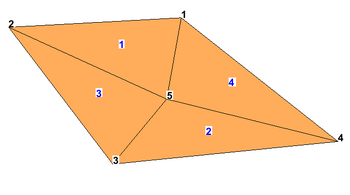
Example 1: 2D UGrid from selecting "Top"


The next two figures show the numbering of the points and cells on the bottom of the 3D UGrid, and on the 2D UGrid that would get generated by the tool if the "Bottom" option is selected. Notice the 2D UGrid numbering differs from the bottom of the 3D UGrid but the order for both points and cells is the same.
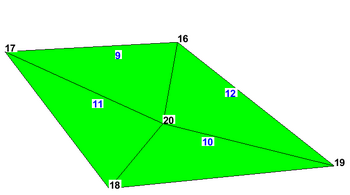
Example 1: 3D UGrid bottom numbering

Example 1: 2D UGrid from selecting "Bottom"


Export Curvilinear Grid
The Export Curvilinear Grid tool is used to create a curvilinear (boundary fitted) grid file (or files) for a curvilinear compatible mesh, scatter set or UGrid that is loaded into SMS. This can make use of user provided I,J index data sets if they exist. It also supports the option to compute I,J data indices. In this case, the orientation of the first cell in the surface will define the orientation of the I,J axes of the grid.
For EFDC grid files it may also use provided cell based datasets to populate the additional properties of the grid. These can include:
- Depth
- Z Roughness
- Vegetation type
- Wind shelter
Input Parameters
The format of the data file will be in either CH3D (also referred to as GSMB) or EFDC (also referred to as LTFATE). The input parameters include:
- Generate cell i-j datasets toggle.
- Cell i-coordinate dataset (optional) – Select the cell based dataset that defines the I index of each cell. This is required if the toggle to generate I-J is not selected.
- Cell j-coordinate dataset (optional) – Select the cell based dataset that defines the J index of each cell. This is required if the toggle to generate I-J is not selected.
Datasets that are available if the format is EFDC:
- Depth dataset (optional) – Select the cell based dataset to define the depth of each cell.
- Z Roughness dataset (optional) – Select the cell based to define the roughness of each cell.
- Vegetation type dataset (optional) – Select the cell based to define the vegetation type of each cell.
- Wind shelter dataset (optional) – Select the cell based to define the wind shelter value of each cell.
Output Parameters
The path to where files will be saved defaults to the project directory if one is defined in the instance of SMS. The path can be cut/paste from a file browser in windows to this edit field.
- CH3D grid file name defaults to "grid.inp".
- EFDC dxdy file name defaults to "dxdy.inp".
- EFDC lxly file name defaults to "lxly.inp".
- EFDC cell file name defaults to "cell.inp".
Current location in toolbox
This tool is currently located in Unstructured Grids/Export Curvilinear Grid.
Notes
The file formats for the CH3D and EFDC grids are defined in the Import Curvilinear Tool documentation. The cell.inp file for EFDC is not used for importing since it does not include any unique information for the definition of the grid. This file includes an ASCII map of the cell types in the grid.
Extrude UGrid
The Extrude UGrid tool converts a 2D UGrid into a 3D UGrid.
Input Parameters
- Input grid – Select a 2D UGrid to convert to a 3D UGrid.
- Number of layers – Enter the number of layers the new 3D UGrid will have.
- Layer n thickness – For each layer, enter the layer thickness. This value will be in the units set in the project projection.
Output Parameters
- Output grid – Name of the output grid.
Current Location in Toolbox
Unstructured Grids/Extrude UGrid
Fill Holes in UGrid
The Fill Holes in UGrid fills all voids in a given mesh with new mesh elements. The output is a mesh that can be converted back into a UGrid if needed. This tool also works on meshes.
Input Parameters
- 2D UGrid – Select a 2D UGrid that needs holes filled.
Output Parameters
- New Mesh Name – Enter the name that the output mesh should have.
Current Location in Toolbox
Unstructured Grids/Fill Holes in UGrid
Import Curvilinear Grid
The Import Curvilinear Grid tool is used to load an existing curvilinear (boundary fitted) grid into SMS as a UGrid object. This will also create cell based datasets defining the I, J index of each cell in the UGrid. Depending on the selected format and the specific data file(s).
For EFDC grid files it may also create additional cell based datasets for the UGrid that is loaded. These can include:
- Depth
- Z Roughness
- Vegetation type
- Wind shelter
Input parameters
- Format of the data file – Select the file format for the UGrid that will be imported.
- "CH3D" – Will import a CH3D file.
- "EFDC" – Will import a EFDC file.
- CH3D formatted grid file – Clicking the Select File button will open a Select File dialog where the CH3D file can be selected.
- EFDC formatted dxdy.inp file – Clicking the Select File button will open a Select File dialog where the dxyy.inp EFDC file can be selected.
- EFDC formatted lxly.inp file – Clicking the Select File button will open a Select File dialog where the lxly.inp EFDC file can be selected.
Output parameters
- Output UGrid name – Enter the name of the imported UGrid.
Current location in the toolbox
Unstructured Grids/Import Curvilinear Grid
CH3D Format
Format of the CH3D file (grid.inp). This file includes a 2 line header and a line for every corner point in a rectangular grid This includes inactive regions. The locations are ordered in a row major order. SMS will export 5 columns of data including (X, Y, Z, I, J). The (I, J) columns are not used in the import process. They are implied. The first line is a name to assign to the grid.
The second line defines the size of the grid based on cell corners. The number of cells in each direction is a maximum of the number of corners minus 1. Cell corners that do not correspond to an active cell in the grid is assigned a coordinate location of (9.0x10¹⁸, 9.0x10¹⁸, 9.0x10¹⁸).
Because this file format does not include cell based information, a single row or column of inactive cells is not supported. The corners of these cells are defined by the active neighbor, so the cell is assumed to exist. File organization:
    Grid_name
    num_rows_of_pts  num_cols_of_pts
    x y z 1 1
    x y z 2 1
    .
    .
    .
    x y z num_rows 1
    x y z 1 2
    x y z 2 2
    .
    .
    .
    x y z num_rows 2
    .
    .
    .
    x y z 1 num
Format of the EFDC files (dxdy.inp, lxly.inp). This format includes two files that work together to define the grid. The "dxdy.inp" files includes a 4 line comment header and a line for every active cell in the grid The header is metadata only and is not used in the import process. The last header line defines the values in each column for the data following. This includes:
- I J: the column and row index of the cell on this line.
- DX DY: the width and height of this cell.
- WATER DEPTH: the depth of the water in this cell.
- BOTTOM ELEV: the ground elevation value for this cell (cell based).
- ZROUGH: the roughness for this cell.
- VEG TYPE: the vegetation type for this cell.
The "lxly.inp" files also includes a 4 line comment header and a line for every active cell in the grid The header is metadata only and is not used in the import process. The last header line defines the values in each column for the data following. This includes:
- I J: the column and row index of the cell on this line.
- X Y: the location of the cell center of this cell.
- CUE CVE CUN CVN: the orientation of this cell (rotation values)
- WIND SHELTER: a wind shelter data value for this cell.
This format defines a nonconformal grid. Neighboring cells don't explicitly define the same corner points. When SMS loads this grid, the corner locations are merged to create a conformal grid. For this reason, when a grid is loaded and then rewritten, the detail definition may not be identical.
Import UGrid Points
The Import UGrid Points tool is used to import locations and datasets. The CSV file must contain coordinates for the points and, optionally, the file may contain datasets associated with the points.
The first line of the CSV file must be a header line with the coordinate columns of x, y, and z (optional). These columns must be named x, y, z. An error will be encountered if these columns do not exist.
Other columns may exist in the file for datasets. The dataset name is specified in the first line of the file. If the column does not have a name then the column will be skipped.
Transient data may also be imported using this tool. Transient datasets comprise multiple columns in the file with the same column name and with time specified on the second line of the file in the associated dataset column. There may not be any value specified on the second line of the file for the x, y coordinates. The time values may be relative times: 0.0, 2.5, 10.0, etc. Additionally, the time values may be specified as date times. The date format should be in the form of YEAR-MONTH-DAY HH:MM:SS.SS.
Multiple example files are shown below.
Input parameters
- CSV file with point coordinates and datasets – Shows the file name for the CSV file containing the coordinates and datasets. Clicking the Select File button will open a Select File browser dialog to select the CSV file.
- No data value – When the “No data value” is encountered in the csv file in one of the datasets XMS marks the value as “NULL” or “no data”. These values are not contoured or used in interpolation in XMS.
- Time unit – The time unit for transient datasets where the time is specified as a floating point number (in contrast to a date time).
- Coordinate system project file (*.prj) – Shows the file name for the projection associated with the coordinates of the points in the file. Clicking the Select File button will open a Select File browser dialog to select the PRJ file.
Current location in Toolbox
Unstructured Grids/Import UGrid Points
Example files
Example 1
id,y,x,c
1,15459458,2685809,6.4
2,15459506,2685824,9.7
3,15459524,2685850,8
This is a simple csv file. Notice the “x” and “y” columns; these are required. Note that “z” is not required. Also, notice that the order of x and y does not matter.
The other 2 columns: “id”, “c”. The will be imported as datasets.
Example 2
y	x	z	TDS	TDS	conc
			0	1
-16	-75	8.5	59.04	9.24	1.9
32	-60	9.8	90.2	71	4.8
50	-34	0.7	67.2	98.4	9.5
This example shows a file with “x”, ”y”, and “z” columns. Notice that there are no values on the second line of the file for x, y, and z. This indicates that times are being specified for the datasets in the file.
The other 2 columns: “TDS” and “conc”. The will be imported as datasets. TDS will be a transient dataset with times of 0.0 and 1.0. The user will have to specify the units of the times in the tool. The conc dataset will be imported without multiple time steps.
Example 3
y	x	c2	c2	c2
		2011-02-01	2012-02-01	2013-02-01
-16	-75	59.04	43.64	9.24
32	-60	90.2	44.16	71
50	-34	67.2	0	98.4
This is a csv file with a transient dataset with the time specified as dates.
Example 4
y	X	c2	c2	c2
		2011-02-01 15:30:22.1	2012-02-01	2013-02-01 6:45:15
-16	-75	59.04	43.64	9.24
32	-60	90.2	44.16	71
50	-34	67.2	0	98.4
This is a csv file with a transient dataset with the time specified as dates and times.
Lloyd Optimizer
The Lloyd Optimizer tool optimizes the angles in a triangular grid to make them close to 60 degrees. It can run for a given time, number of iterations, or until a point no longer moves far. It can also require that all points move far enough.
From CGAL:
This optimization process alternates relocating vertices to the center of mass of their Voronoi cells, and updating the Delaunay connectivity of the triangulation. The center of mass is computed with respect to a sizing function that was designed to preserve the local density of points in the grid...
Input Parameters
- Input grid – A UGrid containing triangles to optimize.
- Number of iterations to perform – The maximum number of iterations to perform before stopping. Can be set to 0 for no limit.
- Maximum duration, in seconds – The maximum amount of time to optimize for, in seconds. Set to "0" for no limit.
- Minimum movement ratio – Fraction of the length of a vertex's shortest incident edge by which it must move during an iteration. If an iteration would move the vertex by less than this amount, then movement of the vertex will be skipped during this iteration. Other vertices may still move during the iteration, and the skipped vertex may be moved during a later iteration if the vertex gets a larger proposed move. This can be useful to prevent the optimizer from spending time moving vertices by tiny amounts. It should be a value between 0 and 1. A value of 0 will disable this condition.
- Freeze ratio – Similar to Move ratio, except that the optimization will stop rather than skip the move.
Additional Notes
The optimizer will not move points on boundary polygons or the boundaries of holes.
During development, points were observed moving across boundaries in some cases. This issue can no longer be reproduced, which prevents understanding the underlying cause and verifying that it is truly resolved. To be on the safe side, the tool will delete any points that migrate across boundaries during optimization.
While this tool operates on any 2D UGrid, it requires that the grid be fully triangulated. To accomodate this, the tool will generate a triangulated grid based on the input grid and optimize the triangulated grid instead. This may result in swapped interior edges and non-triangular cells being broken down into triangular ones. Boundaries and holes will still be preserved.
The optimizer requires that either the Timeout option, number of Iterations option, or both be set to a nonzero value to ensure it converges. If the chosen values prove too low, it is possible to resume the optimization where it left off to save time. To resume optimization, run the tool again and use the previous output grid as the new input grid.
Output Parameters
- Smoothed grid – Name of the output grid.
Current Location in Toolbox
Unstructured Grids/Lloyd Optimizer
Map Activity to UGrid
This tool builds a dataset with values copied from one dataset and activity mapped from another. The tool has the following options:
Input Parameters
- Input grid– Select the geometry that will define the values for the new UGrid.
- Activity coverage – Select the coverage that will define the activity for the new UGrid.
Output Paramters
- Name of the output ugrid – Enter the name for the new activity UGrid.
Current Location in Toolbox
Unstructured Grids/Map Activity to UGrid
Merge 2D UGrids
The Merge 2D UGrids tool merges two 2D geometries. These can be 2D meshes, 2D Grids, UGrids, or scatter sets. The geometries can overlap or not. In areas of overlap, the tool honors the primary grid, deletes all elements from the secondary grid that overlap part of the primary grid plus a buffer around the primary grid. This prevents the transition zone from becoming so small that poorly shaped cells result. The tool builds transition triangle cells to fill the gap created in this process. The new geometry is created as a 2D Mesh in SMS; in GMS, the tool output is a 2D UGrid.
Limitations:
- This tool only works on 2 geometries at a time. If multiple geometries are to be merged, they must be merged incrementally.
- The Primary grid must have defined cells/elements. Any disjoint points on the primary grid will be removed.
This tool is designed to replace the functionality to merge meshes and scatter sets in SMS. This operation is faster, more generic, and because it is in the toolbox, will be accessible outside of the standard SMS framework.
Input parameters
- Primary grid – Select the grid that will act as the primary grid. If there are conflicts during the merge, this grid will receive priority to resolve the conflict.
- Secondary grid – Select the grid that will act as the secondary grid during the merge.
- Duplicate point tolerance – When points are compared as duplicates the distance between the points is calculated. If the distance is less than this tolerance then the points are considered duplicates. This is used for comparing points on the outer boundary of the primary grid with points in the secondary grid and trying to preserve cells in the secondary grid that are adjacent to cells in the primary grid. The default value is usually sufficient but if you find cells in the secondary grid are being deleted and you want to preserve those then try increasing the tolerance.
- Buffer distance option – Option for buffering the outer boundary of the primary grid during the merge operation.
- Default – The tool will use 0.01 times the minimum cell edge length as the buffer distance.
- Specified – The tool will use the user specified buffer distance.
- Buffer distance – specify the desired buffer distance. This is the width of the transition zone between the geomtries.
- Stitch non-overlapping grids with matching boundary points – Option for merging two grids that have matching boundary points and no overlapping features. This option should only be used if the user is positive that the grids satisfy this constraint. A grid with internal holes will result from using this option when the grids overlap. The tool will run significantly faster if this option is checked.
Output parameters
- Merged grid – Enter the name of the new merged UGrid.
Current Location in toolbox
Unstructured Grids/Merge 2D UGrids
Refine UGrid
The Refine UGrid tool creates a 2D UGrid that has been refined based on an existing 2D UGrid and one or more elevation rasters.
Input parameters
- Grid – Select the 2D UGrid that will be refined.
- Default constant value – Enter a value for the desired average cell size for the new UGrid. It is important to note that the tool will refine the entire grid. If the default value is too small then there may be a long computation time for the tool. Entering a value that is too large may cause an error.
- Error threshold – Enter a value to guide the acceptable threshold for error for the grid refinement.
- Maximum iterations – The tool will perform multiple iterations when refining the new UGrid. Enter the maximum number of iterations to perform. The tool will stop performing iterations once it has reached the maximum limit if it has not completed refinement before this value is reached.
- Raster 1 (highest priority) – The elevation raster that will be used for refinement. This raster will be given priority over any additional rasters being used.
- Raster n – Allows selecting an additional raster to use in refinement.
Output parameters
- Output UGrid name – Enter the name for the new refined UGrid.
Current Location in toolbox
Unstructured Grids/Refine UGrid
- It is recommended to use the Smooth Datasets tool instead of this tool.
Smooth UGrid
The Smooth UGrid tool is nearly identical to part of the Smooth Datasets tool. It can be applied to a 2D mesh, a scatter set, or a 2D Ugrid. The tool only supports the slope limited smoothing as described in Smooth Datasets with a user specified anchor type.
The difference between the tools is that this tool actually creates a new geometry with the elevation values smoothed rather than just creating a new dataset on the existing geometry.
Input parameters
- Input grid – Select the UGrid to use.
- Maximum slope – Set the maximum potential slope of the UGrid.
- Anchor type – Select which type of anchor for the smoothing process.
- "Minimum value" – Sets the minimum elevation to be the anchor for the smoothing process.
- "Maximum value" – Sets the maximum elevation to be the anchor for the smoothing process.
Output parameters
- Smoothed grid – Enter the name of the new smoothed UGrid.
Current Location in toolbox
Unstructured Grids/Smooth Ugrid
Related Tools
UGrid from Coverage
The UGrid from Coverage tool creates a 2D unstructured mesh, or UGrid, from the feature objects on a selected coverage.
Input Parameters
- Coverage – Select map coverage in the project.
Output Parameters
- Name of the output mesh – Enter a name for the new UGrid.
Current Location in Toolbox
Unstructed Grids/UGrid from Coverage
UGrid from Surface
The UGrid from Surface tool creates a new UGrid with copies of all of the datasets on the input mesh, scatter set, or Cartesian grid.
Input parameters
- Input grid – Select the input mesh, scatter set, or Cartesian grid to convert to a UGrid.
Output parameters
- Output grid name – Enter the name of the new Ugrid. If left blank the tool will use the name of the input UGrid.
Current location in Toolbox
Unstructured Grids/UGrid from Surface
Voronoi UGrid from UGrid
The Voronoi UGrid from UGrid tool creates a Voronoi UGrid from an existing geometry (2D Mesh, Scatter Set, or UGrid). The tool uses the centroid of each triangle, element or cell of the input geometry as a node in the resulting Voronoi UGrid. The cells around the edge of the UGrid are created by adding a Voronoi node at the bisection of the boundary edge and connecting that node to the node at the triangle/element/cell centroid.
These meshes can be passed into HEC-RAS 2D for analysis.
Input parameters
- Input grid – Select the geometry that will be converted to a Voronoi UGrid.
Output parameters
- Output grid name – Enter the name for the new Voronoi UGrid. This will be a UGrid because scatter sets and meshes do not support polygonal cells.
Current Location in toolbox
Unstructured Grids/Voronoi UGrid from UGrid
SMS – Surface-water Modeling System | ||
|---|---|---|
| Modules: | 1D Grid • Cartesian Grid • Curvilinear Grid • GIS • Map • Mesh • Particle • Quadtree • Raster • Scatter • UGrid | |
| General Models: | 3D Structure • FVCOM • Generic • PTM | |
| Coastal Models: | ADCIRC • BOUSS-2D • CGWAVE • CMS-Flow • CMS-Wave • GenCade • STWAVE • WAM | |
| Riverine/Estuarine Models: | AdH • HEC-RAS • HYDRO AS-2D • RMA2 • RMA4 • SRH-2D • TUFLOW • TUFLOW FV | |
| Aquaveo • SMS Tutorials • SMS Workflows | ||