SMS:BOUSS-2D
| BOUSS-2D | |
|---|---|
 BOUSS-2D Screenshot | |
| Model Info | |
| Model type | Boussinesq Wave Model for Coastal Regions and Harbors. |
| Developer |
Okey George Nawogu, Ph.D. |
| Web site | BOUSS-2D web site |
| Tutorials |
General Section
Models Section
Several sets of sample problems and case studies are available. These include:
|
BOUSS-2D is a comprehensive model for simulating the propagation and tranformation of waves in coastal regions and harbors based on a time-domain solution of Boussinesq-type equations. It is based on Boussinesq-type equations derived by Okey Nwogu and has been under development since 1993. The equations are depth-integrated for the conservation of mass and momentum for nonlinear waves propagating in shallow and intermediate water depths.
The BOUSS-2D model can be added to a paid edition of SMS.
Functionality
BOUSS-2D computes nearshore wave fields including mean wave heights, mean current direction, mean water level breaking and transient representation of water levels, currents, and wave breaking.
BOUSS-2D is a comprehensive numerical model for simulating the propagation and transformation of waves in coastal regions and harbors based on a time-domain solution of Boussinesq-type equations. The governing equations are uniformly valid from deep to shallow water and can simulate most of the phenomena of interest in the nearshore zone and harbor basins including:
- Reflection/diffraction near structures
- Energy dissipation due to wave breaking and bottom friction
- Cross-spectral energy transfer due to nonlinear wave-wave interactions
- Breaking-induced longshore and rip currents
- Wave-current interaction
- Wave interaction with porous structures
The governing equations in BOUSS-2D are solved in the time domain with a finite-difference method. Input waves may be periodic (regular) or non-periodic (irregular), and both unidirectional or multi-directional sea states may be simulated. Waves propagating out of the computation domain are either absorbed in damping layers or allowed to leave the domain freely. The SI engineering units are used in BOUSS-2D calculations.
Output Options
See Output Options in the BOUSS-2D Simulations article.
Saving BOUSS-2D
When completing a File | Save As... command, the following files get saved in the *.sms
- *.mat referenced to new save location
- *.map referenced to new save location
- Damping files saved to temp folder
- *.par referenced to new save location
- *.sol referenced to original save location unless rerun
- *.h5 referenced to new save location
Using the Model / Practical Notes
BOUSS-2D can be applied to a wide variety of coastal and ocean engineering problems, including complex wave transformation over small coastal regions (1-5 km), wave agitation and harbor resonance studies, wave breaking over submerged obstacles, breaking-induced nearshore circulation patterns, wave-current interaction near tidal inlets, infra-gravity wave generation by groups of short waves, and wave transformation around artificial islands.
As with many numerical models, BOUSS-2D can terminate or crash due to numerical instabilities. These are usually caused by problems related to the grid, the boundary conditions, or model parameters. The following lists describe common causes of instability and methods to correct them.
Instability due to the grid/geometry
- Model stability requires a low Courant number throughout the domain. SMS computes an approximate maximum time step to maintain a Courant number below 0.5. In some cases, it is desired to lower the time step even more. Additionally, some may want to truncate the computational domain to areas with depth above a specified minimum. Another option is to increase resolution by using smaller computational cells. Either of these options increase run time, so before applying them, look at the other causes of instability.
- Abrupt changes in elevation from one cell to another in the computational domain could result in instabilities. It may be helpful to smooth the grid. (A smoothing command is available by right clicking on the grid object in the project explorer in the SMS interface.)
- Computation nodes surrounded on three or four sides by land may be created during the grid creation process. These "isolated" cells may become unstable and generally don't have an impact on the wave climate. They can be converted to land cells.
Instability due to the boundary conditions
- Generally, avoid placing damping or porosity layers along structures and shorelines.
- Wave makers are more stable on the edges of the domain. Therefore, generally speaking, the wave maker should be placed on the boundary of the domain in constant (or nearly constant) depth water. (The SMS interface offers to extend the grid and transition to constant depth if a wave maker is created in a location with more that 20% variation in depth.) This is especially true in real world applications where reflected waves are of no concern. Also, when simulating large waves, the greater stability of external wavemakers may be required.
- Wave makers should be placed far enough from shore to avoid interaction between the wave maker and reflecting waves. This is because the external boundary behind the wave maker is treated as a vertical wall.
- Exceptions, or applications in which internal wavemakers (i.e. wavemakers placed inside the domain) are recommended include:
- In applications with significant reflections from structures inside the computational domain. When reflected are caused by coastlines, structures, or bathymetry (reflected wave sources), the simulated seastate will become less uniform spatially, and the simulation may not reach a steady-state condition. The resulting wave field in such simulations will generally consist of nodes and anti-nodes that resemble a standing wave pattern, where waves appear to be bouncing back and forth inside the domain. If reflected waves cannot escape through boundaries of the modeling domain (or are constrained to exit the domain), a steady-state condition technically cannot be reached irrespective of the length of simulation. When reflected waves intercept external wavemakers, the extremes (lows and highs) in the calculated wavefield may keep building and can eventually lead to model instabilities.
- Internal wavemakers should be used for finite domains and especially for limited area physical modeling studies, and with the above specified guidance.
- If wavemakers are placed on the interior of the domain, they should cross the entire domain to avoid potential "end effects", and have a damping layer placed behind (on the seaward side of) the internal wavemakers to absorb reflected waves. There should also be a gap (at least one non-damped cell) between the internal wavemaker and the damping layer located offshore.
- In the absence of laboratory or field data to calibrate damping and porous layers for an application, consider multiple simulations with a range of damping widths and/or coefficients. This graph from BOUSS-2D's technical report illustrates the variation of effective reflectivity given various damping coefficients and damping layer widths. To use this graph:
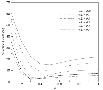
- Compute L (the wavelength for the incident wave).
- Select a w/L ratio. Use this ratio to compute w (damping width).
- Select an expected reflection percentage. Follow a horizontal line for this percentage on plot to intersect the graph for selected w/L ratio. Read associated damping coefficient from plot.
- Note that the reflection coefficient is very sensitive to a change in damping coefficient when the coefficient is small (< 0.3) and much less sensitive when the coefficient is larger.
- This process may require the damping parameters be changed when different wave conditions are considered.
- It should be observed that this plot is for normally incident waves. Different reflection coefficients would be obtained for obliquely incident waves.
- Damping layers should be 5–10 cells wide.

Instability due to model parameters
- The model includes a Smagorinsky term to account for subgrid turbulence. If the turbulence is known, it is expected this term can be left at the default (0.0), however, it may be increased to increase stability. (This should be done with caution. Remember, don't suppress the wiggles, they are trying to say something.)
Test Cases
- Test 1 – Simple test demonstrating the use of an internal wavemaker.
External Links
- BOUSS-2D User Manual
- CHL BOUSS-2D website [1]
- May 2007 ERDC/CHL CHETN-I-73 Infra-Gravity Wave Input Toolbox (IGWT): User’s Guide [2]
- May 2005 ERDC/CHL CHETN-I-70 BOUSS-2D Wave Model in SMS: 2. Tutorial with Examples [3]
- Mar 2005 ERDC/CHL CHETN-I-69 BOUSS-2D Wave Model in the SMS: 1. Graphical Interface [4]
- Aug 2011 Tsunami Modeling Example Study - A Joint Hydraulic/Structural Methodology for the Rehabilitation of the Crescent City Marina [5]
- Apr 2014 Tsunami Modeling Article [6]
Related Topics
- BOUSS-2D Graphical Interface
- Cartesian Grid Module
- BOUSS-2D Files
- BOUSS-2D Model Control Dialog
- BOUSS-2D Calculators
- CGWAVE
- SMS Models page
- Spectral Energy
| [hide] SMS – Surface-water Modeling System | ||
|---|---|---|
| Modules: | 1D Grid • Cartesian Grid • Curvilinear Grid • GIS • Map • Mesh • Particle • Quadtree • Raster • Scatter • UGrid |  |
| General Models: | 3D Structure • FVCOM • Generic • PTM | |
| Coastal Models: | ADCIRC • BOUSS-2D • CGWAVE • CMS-Flow • CMS-Wave • GenCade • STWAVE • WAM | |
| Riverine/Estuarine Models: | AdH • HEC-RAS • HYDRO AS-2D • RMA2 • RMA4 • SRH-2D • TUFLOW • TUFLOW FV | |
| Aquaveo • SMS Tutorials • SMS Workflows | ||