SMS:LTEA: Difference between revisions
mNo edit summary |
m (Protected "SMS:LTEA" ([Edit=Allow only administrators] (indefinite) [Move=Allow only administrators] (indefinite))) |
||
| (92 intermediate revisions by 3 users not shown) | |||
| Line 1: | Line 1: | ||
Linear Truncation Error Analysis (LTEA) was initially presented by Dr. Scott C. Hagen as part of his doctoral research at Notre Dame | <!--*NOTE: This feature will be deprecated in SMS version 13.2. This is the last version of the code that will include this tool. A new python library (pyLTEA) has been under development individuals in the ADCIRC community. Our intent is to include this library as a tool in the SMS python toolbox.--> | ||
{{SMS Deprecated Feature}} | |||
Linear Truncation Error Analysis (LTEA) Toolbox incorporated into SMS uses the LTEA algorithm as the heart of a utility which creates finite element meshes of varying resolution for ADCIRC analysis. The algorithm was initially presented by Dr. Scott C. Hagen as part of his doctoral research at Notre Dame, and development has continued on the methodology at the University of Central Florida. It performs analysis on an existing [[SMS:ADCIRC|ADCIRC]] mesh and its solution to help quantify the error associated with the mesh. | |||
Normally, this [[SMS:ADCIRC|ADCIRC]] solution is taken from a "linear ADCIRC" run. This type of run is used to make the process faster and to simplify the LTEA algorithm applied to the unstructured mesh. A second phase of the LTEA process uses the error values at each node to create a relative size function covering the domain called "Del X". This refines the mesh where the element error values would be greatest such as near shorelines or around islands. | |||
SMS | |||
== Mesh Generation Toolbox Dialog == | |||
[[File:ADCIRC MeshGenerationToolbox.png|thumb|230 px|''Mesh Generation Toolbox'' dialog]] | |||
SMS includes a graphical interface that allows using the LTEA algorithm to guide the generation of a finite element mesh. Before using the tool, ADCIRC must be run in order to generate the datasets necessary for LTEA to run. | |||
The tool requires the following inputs to be in the Project Explorer: | |||
* A bathymetry scatter set. | * A bathymetry scatter set. | ||
* | * A 2D mesh. | ||
* A mesh generation coverage having at least one polygon. | |||
The following may be required, depending on the options selected: | |||
* Harmonic ADCIRC solution dataset(s) | |||
The toolbox is accessed by: | |||
#Right-clicking on the mesh generation coverage and selecting '''Mesh Generation Toolbox...''' to bring up the ''Mesh Generation Toolbox'' dialog. | |||
#Select "Localized Truncation Error Analysis (LTEA)" from the list and click '''Run''' to bring up the ''LTEA Tool'' dialog. | |||
The ''LTEA Tool'' dialog is discussed in the next section. | |||
==LTEA Tool Dialog== | |||
[[File:LTEA Tool dialog first page.png|thumb|right|450 px|The first page in the ''LTEA Tool'' dialog.]] | |||
A set of standard buttons can be found at the bottom of the ''LTEA Tool'' dialog: | |||
*'''Help...''' – Opens [[SMS:LTEA]]. | |||
*'''< Previous''' – Returns to the previous step in the dialog. | |||
*'''Continue >''' – Moves to next step of the dialog. | |||
*'''Stop and Run''' – Closes the dialog and runs LTEA. The analysis generates several datasets used as size functions in the mesh generation process. Visible on all but the final page of the dialog. | |||
*'''Run''' – Runs LTEA at the completion of all steps. Only visible on the ''Generate Final Mesh'' page of the dialog. | |||
*'''Cancel''' – Closes the ''LTEA Tool'' dialog without saving any information entered. | |||
* | The first page of the ''LTEA Tool'' dialog has the following options on the left: | ||
*''Boundary'' – Select the desired coverage from the drop-down. There may be only one option in some cases. | |||
*''Bathymetry'' – Clicking '''Select...''' brings up the ''Select Dataset'' dialog. | |||
**{{anchor|select-dataset}}''Select Dataset'' dialog | |||
***''Select'' section – Select the desired bathymetry dataset from the tree list. | |||
***''Select time step'' section – After selecting the dataset, if the dataset has time steps, select the desired time step or turn on ''All time steps''. | |||
***'''Help...''' – Opens [[SMS:Datasets]]. | |||
***'''Select''' – Closes the ''Select Dataset'' dialog and saves the selected dataset. | |||
***'''Cancel''' – Closes the ''Select Dataset'' dialog without saving any selections. | |||
*''Bathymetry'' – Clicking '''Select...''' brings up the ''Select Dataset'' dialog, where the desired mesh can be selected. | |||
On the right are the following options: | |||
*''Provide harmonic solutions'' | |||
**''Eta amplitude'' – Clicking '''Select...''' brings up the ''Select Dataset'' dialog, where the desired eta amplitude dataset can be selected. | |||
**''Eta phase'' – Clicking '''Select...''' brings up the ''Select Dataset'' dialog, where the desired eta phase dataset can be selected. | |||
**''Velocity amplitude'' – Clicking '''Select...''' brings up the ''Select Dataset'' dialog, where the desired velocity amplitude dataset can be selected. | |||
**''Velocity phase'' – Clicking '''Select...''' brings up the ''Select Dataset'' dialog, where the desired velocity phase dataset can be selected. | |||
*''Provide Del X'' | |||
**''Del X'' – Clicking '''Select...''' brings up the ''Select Dataset'' dialog, where the desired Del X dataset can be selected. | |||
If the ''Provide harmonic solutions'' option is selected and '''Continue >''' is clicked, the [[#LTEA Tool → LTEA|''LTEA'' page]] of the dialog will come up. If ''Provide Del X'' is selected and '''Continue >''' is clicked, the [[#LTEA Tool → Generate Final Mesh|''Generate Final Mesh'' page]] of the dialog will come up. | |||
* | ===LTEA Tool → LTEA === | ||
[[File:LTEA Tool dialog Run Type page.png|thumb|right|450 px|The second page in the ''LTEA Tool'' dialog after selecting ''Provide harmonic solutions''.]] | |||
There are several options on the ''LTEA'' page of the ''LTEA Tool'' dialog. This page is reached after selecting ''Provide harmonic solutions'' on the first page. | |||
*''LTEA'' section | |||
**''Run type'' drop-down – Select from the following options: | |||
***"LTEA" – Local Truncation Error Analysis | |||
***"LTEACD" – Local Truncation Error Analysis with Complex Derivatives. | |||
**''Value for dx'' – Decimal value for dx. | |||
**''Minimum spacing from'' – Normally grayed out. | |||
**''Node number'' – Normally grayed out. | |||
**''Use partial molecule'' – Not available if "LTEACD" selected from ''Run type'' drop-down. If turned on, LTEA will give values for nodes with partial molecules. If turned off, LTEA will only give values for nodes completely within the domain. | |||
**''Molecule size'' drop-down – Contains one or more possible molecule sizes. | |||
***"9 x 9" – a small, equally-spaced grid of nine cells by nine cells is created around each node, and values from the ADCIRC solutions are interpolated for all 81 cells. | |||
The | ===LTEA Tool → Generate Final Mesh=== | ||
[[File:LTEA Tool dialog Generate Final Mesh.png|thumb|right|450 px|The third page in the ''LTEA Tool'' dialog after selecting ''Provide Del X''.]] | |||
The ''Generate Final Mesh'' is reached by continuing after either selecting ''Provide Del X'' on the first page of the ''LTEA Tool'' dialog or by continuing after the ''LTEA'' page of the dialog. The options in the ''Generate Final Mesh'' section include: | |||
*''Target number of nodes'' – Fill in the target number of nodes (x) and a value for ''plus/minus'' the number of nodes (y). This gives a range of "x ± y" targeted nodes. | |||
*''Element area change limit'' – A decimal value for the element area change limit. | |||
*''Redistribute boundaries'' – Turn on to redistribute boundaries. | |||
*''Truncate element sizes'' – Turn on to truncate element sizes according to the minimum and maximum specified. | |||
**''Minimum size'' – Minimum element size in project units | |||
**''Maximum size'' – Maximum element size in project units | |||
== Case Studies / Sample Problems == | == Case Studies / Sample Problems == | ||
=== | === Tutorials === | ||
The following [[SMS:Tutorials|tutorials]] may be helpful for learning to use LTEA in SMS: | The following [[SMS:Tutorials|tutorials]] may be helpful for learning to use LTEA in SMS: | ||
* Models Section | * Models Section | ||
** ADCIRC LTEA | ** ADCIRC LTEA – Uses LTEA to mesh Shinnecock bay and the area around it along Long Island, NY. | ||
=== American Samoa === | === American Samoa === | ||
The following images illustrate the results of the LTEA toolbox applied to a domain around American Samoa. The first pair of images illustrate a mesh generated for the domain using the paving method. Density at the coastline was controlled by redistributing the vertices on the arcs representing the coastline and the density varied to a larger ocean boundary density. This mesh consists of 22,576 nodes (43,055 elements). The other images illustrate the varying resolution generated by LTEA to result in constant error with target mesh sizes of 24,000 nodes and 12,000 nodes respectively. The LTEA toolbox created meshes with 24,078 nodes (45,929 elements) and 12,029 nodes ( 22,543 elements). | |||
<gallery widths="240px" heights="160px" perrow="5"> | |||
Image:AmericanSamoaPaved.jpg|Paved Mesh | |||
Image:AmericanSamoaLT24K.jpg|24000 Node Mesh | |||
Image:AmericanSamoaLT12K.jpg|12000 Node Mesh | |||
Image:AmericanSamoaPaved_Zoom.jpg|Paved Mesh Detail | |||
Image:AmericanSamoaLT24K_Zoom.jpg|24000 Node Detail | |||
Image:AmericanSamoaLT12K_Zoom.jpg|12000 Node Detail | |||
</gallery> | |||
These images illustrate the redistribution of density to increase the density in areas that require additional detail for solution variations, or to reduce the number of nodes in the mesh. | |||
=== Glacier Bay Alaska === | === Glacier Bay Alaska === | ||
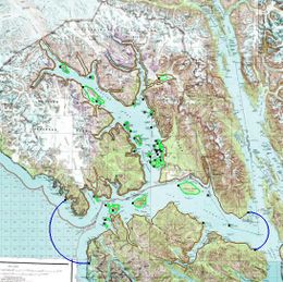
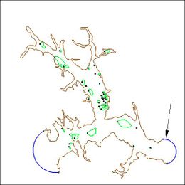
The case of [http://water.engr.psu.edu/hill/research/glba/default.stm Glacier Bay Alaska], by [http://water.engr.psu.edu/hill/default.stm Dave F. Hill's] research group, poses another problem for the LTEA toolbox. This case includes two ocean boundaries. The figures below show three meshes generated for this case and illustrate the large variation in node density that can be produced by the procedure. | |||
<gallery widths="260px" heights="260px"> | |||
Image:GlacierBayImage.jpg|Glacier Bay Domain over areal photo | |||
Image:GlacierBayConceptual.jpg|Glacier Bay Domain with second ocean boundary highlighted | |||
</gallery> | |||
This case includes two ocean boundaries. Currently, the LTEA toolbox makes a sometimes erroneous assumption that only one ocean boundary exists. To work around this problem in the current version of SMS, the following steps are required: | |||
* Change the inland ocean boundary to land | * Change the inland ocean boundary to land | ||
* Run the first step of the LTEA toolbox to generate the "Linear Run Mesh" and then "Stop and Run" to that point. | * Run the first step of the LTEA toolbox to generate the "Linear Run Mesh" and then "Stop and Run" to that point. | ||
[[Image:GlacierBayLiinear.jpg|200px | {| | ||
[[Image:LTEA_Harmonics. | |- | ||
* Outside of the toolbox, change the second ocean boundary to ocean on the linear run mesh and run a linear run of ADCIRC with harmonic analysis turned on. This will generate the | |[[Image:GlacierBayLiinear.jpg|thumb|200px|Linear mesh for Glacier Bay (17,717 nodes)]] | ||
|valign="top"|[[Image:LTEA_Harmonics.png|thumb|250px|Harmonic datasets for LTEA analysis]] | |||
|} | |||
* Outside of the toolbox, change the second ocean boundary to ocean on the linear run mesh and run a linear run of ADCIRC with harmonic analysis turned on. This will generate the datasets for LTEA calcuations. | |||
* Relaunch the toolbox and select the datasets from the linear run to guide the mesh generation process. | * Relaunch the toolbox and select the datasets from the linear run to guide the mesh generation process. | ||
<gallery widths="260px" heights="240px" perrow="5"> | |||
Image:GlacierBay10K.jpg|20000 Node Mesh (19,929 nodes) | |||
Image:GlacierBay20K.jpg|20000 Node Mesh (30,227 nodes) | |||
Image:GlacierBay30K.jpg|30000 Node Mesh (10,072 nodes) | |||
</gallery> | |||
== Related Topics == | == Related Topics == | ||
* [[SMS:ADCIRC|ADCIRC]] | * [[SMS:ADCIRC|ADCIRC]] | ||
* [[SMS:Steering|Steering]] | * [[SMS:Steering|Steering]] | ||
* [[ADCIRC LTEA Workflow|ADCIRC LTEA Workflow]] | |||
== | == Additional Reading == | ||
* [http://champs.cecs.ucf.edu/ Coastal Hydroscience Analysis, Modeling & Predictive Simulations Laboratory (CHAMPS Lab)] | * [http://champs.cecs.ucf.edu/ Coastal Hydroscience Analysis, Modeling & Predictive Simulations Laboratory (CHAMPS Lab)] | ||
* [http:// | * [http://scholarsarchive.byu.edu/cgi/viewcontent.cgi?article=1780&context=etd Sep 2006 Automatic, unstructured mesh generation for 2D, shelf-based tidal models] | ||
* [http://champs.cecs.ucf.edu/Publications/Refereed/IJCFD_Hagen_et_al_2006.pdf Sep 2006 Automatic, unstructured mesh generation for tidal calculations in a large domain] | * [http://champs.cecs.ucf.edu/Publications/Refereed/IJCFD_Hagen_et_al_2006.pdf Sep 2006 Automatic, unstructured mesh generation for tidal calculations in a large domain] | ||
* [http://poc.omp.obs-mip.fr/DOCUMENTS/t-ugo/res.pdf Sep 2006 Resolution Issues in Numerical Models of Oceanic and Coastal Circulation] | * [http://poc.omp.obs-mip.fr/DOCUMENTS/t-ugo/res.pdf Sep 2006 Resolution Issues in Numerical Models of Oceanic and Coastal Circulation] | ||
* [http://www.nd.edu/~adcirc/pubs/IJNMF-hwkh-2001-PUBL.pdf 2001 Two-dimensional, unstructured mesh generation for tidal models] | * [http://www.nd.edu/~adcirc/pubs/IJNMF-hwkh-2001-PUBL.pdf 2001 Two-dimensional, unstructured mesh generation for tidal models] | ||
* [http://www.nd.edu/~adcirc/pubs/ijnmf-hwk-2000-PUBL.pdf 2000 One-dimensional finite element grids based on a localized truncation error analysis] | * [http://www.nd.edu/~adcirc/pubs/ijnmf-hwk-2000-PUBL.pdf 2000 One-dimensional finite element grids based on a localized truncation error analysis] | ||
* [http://water.engr.psu.edu/hill/research/glba/default.stm Glacier Bay Test Case by Dave F. Hill] | * [http://water.engr.psu.edu/hill/research/glba/default.stm Glacier Bay Test Case by Dave F. Hill] | ||
{{Template: | |||
{{Template:Navbox SMS}} | |||
[[Category:ADCIRC Dialogs]] | |||
[[Category:ADCIRC|L]] | |||
[[Category:External Links]] | |||
Latest revision as of 18:50, 24 March 2023
| This contains information about features no longer in use for the current release of SMS. The content may not apply to current versions. |
Linear Truncation Error Analysis (LTEA) Toolbox incorporated into SMS uses the LTEA algorithm as the heart of a utility which creates finite element meshes of varying resolution for ADCIRC analysis. The algorithm was initially presented by Dr. Scott C. Hagen as part of his doctoral research at Notre Dame, and development has continued on the methodology at the University of Central Florida. It performs analysis on an existing ADCIRC mesh and its solution to help quantify the error associated with the mesh.
Normally, this ADCIRC solution is taken from a "linear ADCIRC" run. This type of run is used to make the process faster and to simplify the LTEA algorithm applied to the unstructured mesh. A second phase of the LTEA process uses the error values at each node to create a relative size function covering the domain called "Del X". This refines the mesh where the element error values would be greatest such as near shorelines or around islands.
Mesh Generation Toolbox Dialog

SMS includes a graphical interface that allows using the LTEA algorithm to guide the generation of a finite element mesh. Before using the tool, ADCIRC must be run in order to generate the datasets necessary for LTEA to run.
The tool requires the following inputs to be in the Project Explorer:
- A bathymetry scatter set.
- A 2D mesh.
- A mesh generation coverage having at least one polygon.
The following may be required, depending on the options selected:
- Harmonic ADCIRC solution dataset(s)
The toolbox is accessed by:
- Right-clicking on the mesh generation coverage and selecting Mesh Generation Toolbox... to bring up the Mesh Generation Toolbox dialog.
- Select "Localized Truncation Error Analysis (LTEA)" from the list and click Run to bring up the LTEA Tool dialog.
The LTEA Tool dialog is discussed in the next section.
LTEA Tool Dialog

A set of standard buttons can be found at the bottom of the LTEA Tool dialog:
- Help... – Opens SMS:LTEA.
- < Previous – Returns to the previous step in the dialog.
- Continue > – Moves to next step of the dialog.
- Stop and Run – Closes the dialog and runs LTEA. The analysis generates several datasets used as size functions in the mesh generation process. Visible on all but the final page of the dialog.
- Run – Runs LTEA at the completion of all steps. Only visible on the Generate Final Mesh page of the dialog.
- Cancel – Closes the LTEA Tool dialog without saving any information entered.
The first page of the LTEA Tool dialog has the following options on the left:
- Boundary – Select the desired coverage from the drop-down. There may be only one option in some cases.
- Bathymetry – Clicking Select... brings up the Select Dataset dialog.
- Select Dataset dialog
- Select section – Select the desired bathymetry dataset from the tree list.
- Select time step section – After selecting the dataset, if the dataset has time steps, select the desired time step or turn on All time steps.
- Help... – Opens SMS:Datasets.
- Select – Closes the Select Dataset dialog and saves the selected dataset.
- Cancel – Closes the Select Dataset dialog without saving any selections.
- Select Dataset dialog
- Bathymetry – Clicking Select... brings up the Select Dataset dialog, where the desired mesh can be selected.
On the right are the following options:
- Provide harmonic solutions
- Eta amplitude – Clicking Select... brings up the Select Dataset dialog, where the desired eta amplitude dataset can be selected.
- Eta phase – Clicking Select... brings up the Select Dataset dialog, where the desired eta phase dataset can be selected.
- Velocity amplitude – Clicking Select... brings up the Select Dataset dialog, where the desired velocity amplitude dataset can be selected.
- Velocity phase – Clicking Select... brings up the Select Dataset dialog, where the desired velocity phase dataset can be selected.
- Provide Del X
- Del X – Clicking Select... brings up the Select Dataset dialog, where the desired Del X dataset can be selected.
If the Provide harmonic solutions option is selected and Continue > is clicked, the LTEA page of the dialog will come up. If Provide Del X is selected and Continue > is clicked, the Generate Final Mesh page of the dialog will come up.
LTEA Tool → LTEA

There are several options on the LTEA page of the LTEA Tool dialog. This page is reached after selecting Provide harmonic solutions on the first page.
- LTEA section
- Run type drop-down – Select from the following options:
- "LTEA" – Local Truncation Error Analysis
- "LTEACD" – Local Truncation Error Analysis with Complex Derivatives.
- Value for dx – Decimal value for dx.
- Minimum spacing from – Normally grayed out.
- Node number – Normally grayed out.
- Use partial molecule – Not available if "LTEACD" selected from Run type drop-down. If turned on, LTEA will give values for nodes with partial molecules. If turned off, LTEA will only give values for nodes completely within the domain.
- Molecule size drop-down – Contains one or more possible molecule sizes.
- "9 x 9" – a small, equally-spaced grid of nine cells by nine cells is created around each node, and values from the ADCIRC solutions are interpolated for all 81 cells.
- Run type drop-down – Select from the following options:
LTEA Tool → Generate Final Mesh

The Generate Final Mesh is reached by continuing after either selecting Provide Del X on the first page of the LTEA Tool dialog or by continuing after the LTEA page of the dialog. The options in the Generate Final Mesh section include:
- Target number of nodes – Fill in the target number of nodes (x) and a value for plus/minus the number of nodes (y). This gives a range of "x ± y" targeted nodes.
- Element area change limit – A decimal value for the element area change limit.
- Redistribute boundaries – Turn on to redistribute boundaries.
- Truncate element sizes – Turn on to truncate element sizes according to the minimum and maximum specified.
- Minimum size – Minimum element size in project units
- Maximum size – Maximum element size in project units
Case Studies / Sample Problems
Tutorials
The following tutorials may be helpful for learning to use LTEA in SMS:
- Models Section
- ADCIRC LTEA – Uses LTEA to mesh Shinnecock bay and the area around it along Long Island, NY.
American Samoa
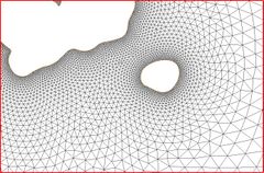
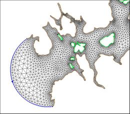
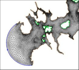
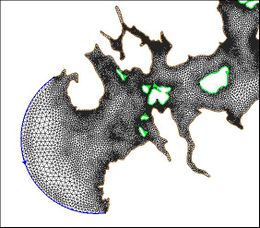
The following images illustrate the results of the LTEA toolbox applied to a domain around American Samoa. The first pair of images illustrate a mesh generated for the domain using the paving method. Density at the coastline was controlled by redistributing the vertices on the arcs representing the coastline and the density varied to a larger ocean boundary density. This mesh consists of 22,576 nodes (43,055 elements). The other images illustrate the varying resolution generated by LTEA to result in constant error with target mesh sizes of 24,000 nodes and 12,000 nodes respectively. The LTEA toolbox created meshes with 24,078 nodes (45,929 elements) and 12,029 nodes ( 22,543 elements).
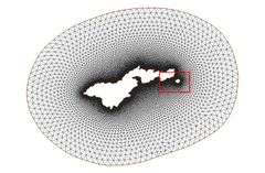
Paved Mesh
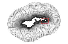
24000 Node Mesh
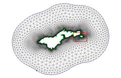
12000 Node Mesh
Paved Mesh Detail
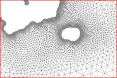
24000 Node Detail
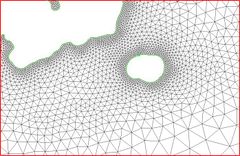
12000 Node Detail


These images illustrate the redistribution of density to increase the density in areas that require additional detail for solution variations, or to reduce the number of nodes in the mesh.
Glacier Bay Alaska
The case of Glacier Bay Alaska, by Dave F. Hill's research group, poses another problem for the LTEA toolbox. This case includes two ocean boundaries. The figures below show three meshes generated for this case and illustrate the large variation in node density that can be produced by the procedure.
Glacier Bay Domain over areal photo
Glacier Bay Domain with second ocean boundary highlighted


This case includes two ocean boundaries. Currently, the LTEA toolbox makes a sometimes erroneous assumption that only one ocean boundary exists. To work around this problem in the current version of SMS, the following steps are required:
- Change the inland ocean boundary to land
- Run the first step of the LTEA toolbox to generate the "Linear Run Mesh" and then "Stop and Run" to that point.


- Outside of the toolbox, change the second ocean boundary to ocean on the linear run mesh and run a linear run of ADCIRC with harmonic analysis turned on. This will generate the datasets for LTEA calcuations.
- Relaunch the toolbox and select the datasets from the linear run to guide the mesh generation process.
20000 Node Mesh (19,929 nodes)
20000 Node Mesh (30,227 nodes)
30000 Node Mesh (10,072 nodes)


Related Topics
Additional Reading
- Coastal Hydroscience Analysis, Modeling & Predictive Simulations Laboratory (CHAMPS Lab)
- Sep 2006 Automatic, unstructured mesh generation for 2D, shelf-based tidal models
- Sep 2006 Automatic, unstructured mesh generation for tidal calculations in a large domain
- Sep 2006 Resolution Issues in Numerical Models of Oceanic and Coastal Circulation
- 2001 Two-dimensional, unstructured mesh generation for tidal models
- 2000 One-dimensional finite element grids based on a localized truncation error analysis
- Glacier Bay Test Case by Dave F. Hill
SMS – Surface-water Modeling System | ||
|---|---|---|
| Modules: | 1D Grid • Cartesian Grid • Curvilinear Grid • GIS • Map • Mesh • Particle • Quadtree • Raster • Scatter • UGrid |  |
| General Models: | 3D Structure • FVCOM • Generic • PTM | |
| Coastal Models: | ADCIRC • BOUSS-2D • CGWAVE • CMS-Flow • CMS-Wave • GenCade • STWAVE • WAM | |
| Riverine/Estuarine Models: | AdH • HEC-RAS • HYDRO AS-2D • RMA2 • RMA4 • SRH-2D • TUFLOW • TUFLOW FV | |
| Aquaveo • SMS Tutorials • SMS Workflows | ||