GMS:Solids to MODFLOW Command
The Solids → MODFLOW command represents a powerful tool for modeling complex stratigraphy in a completely grid-independent fashion. As part of the overall conceptual model building process, the stratigraphy at a site is modeled as a set of solids. The solids are built using tools in the Borehole, TIN, and Solids modules. These solids can represent a wide variety of complex stratigraphic relationships. Then assign hydraulic conductivity (Kh and Kv) and storage coefficients to the solids as material properties and a multi-layer grid is constructed where the boundary of the grid occupies the same region of the solids in plan view. The Solids → MODFLOW command can then be used to automatically define the elevation arrays in MODFLOW. If the grid is refined or edited in any way, this command can be selected again to rebuild the arrays in seconds with no further user intervention. Together with the feature objects in the Map module, a set of solids can be used to build a completely grid-independent conceptual model regardless of the complexity of the site.
Following is the set of steps required to use the Solids → MODFLOW command:
- Building the Solids
- Material Properties
- Creating the Grid
- When using Boundary matching, match layers to solids
- Execute Solids → MODFLOW
Building the Solids
Before executing the Solids → MODFLOW command, a set of solids should be constructed that match the site stratigraphy. These solids are typically constructed using the horizons approach. When building these solids, it is best to build the primary TIN with a larger outer polygon boundary than the boundary that is used to define the MODFLOW conceptual model. This ensures that the stratigraphy will encompass all of the grid.
Material Properties
The next step is to create a set of material properties for the solids using the Material command in the Edit menu.
Creating the Grid
Once the solids are created and the layer assignments are made, the next step is to create a grid. The grid boundary in the xy plane (plan view) should either match the boundary of the solids or encompass the solids. The grid can be refined around wells if desired. The number of layers in the grid should be compatible with the layer assignments made to the solids. When the grid is first created, the z elevations can be ignored since they will be inherited from the solids. A sample grid is shown below.
After the grid is created, the cells outside the model domain should be inactivated using the Activate Cells in Coverage command in Feature Objects menu in the Map module.

Solids → MODFLOW Options

The Solids → MODFLOW command brings up a dialog listing the three basic options associated with the Solids → MODFLOW command. Each option utilizes a different approach for converting the solid stratigraphy to the MODFLOW BCF input arrays. The three options are:
Boundary Matching
One of the three basic options associated with the Solids → MODFLOW command is the Boundary Matching option. The goal of the boundary matching algorithm is to compute a set of elevation arrays that honor the boundaries between the stratigraphic units as closely as possible.
Solids and Layer Ranges
Next a layer range must be assigned to each solid. The layer range represents the consecutive sequence of layer numbers in the MODFLOW grid that are to coincide with the solid model. A sample set of layer range assignments is shown in the figure below (a). The example in the figure below is a case where each solid is continuous through the model domain and there are no pinchouts. Each of the solids is given a layer range defined by a beginning and ending grid layer number. The resulting MODFLOW grid is shown in the figure below (b).

A more complex case with pinchouts is illustrated in the next figure (a). Solid A is given the layer range 1–4, and the enclosed pinchout (solid B) is given the layer range 2–2. The set of grid layers within the defined range that are actually overlapped by the model may change from location to location. The layer range represents the set of grid layers potentially overlapped by the solid anywhere in the model domain. For example, on the left side of the problem shown in the figure below (a), solid A covers grid layers 1, 2, 3 and 4. On the right side of the model, solid A is associated with grid layers 1, 3 and 4 since the enclosed solid (solid B) is associated with layer 2. Likewise, Solid C is associated with grid layers 5 and 6 on the left side of the model but only with layer 6 on the right side of the model where solid D is associated with layer 5. The resulting MODFLOW grid is shown in the figure below (b).

When assigning layer ranges to solids, care must be taken to define associations that are topologically sound. For example, since solid B in the figure above (a) is enclosed by solid A, solid B could not be assigned a layer range that is outside the layer range of solid A.
Layer ranges are assigned using the Solids Properties dialog.
Solids → MODFLOW Command
The final step is to select the Solids → MODFLOW command in the Solids menu. The layer elevations and material properties for the 3D grid will then be automatically assigned from the solids as shown below.

The following images represent cross-sections at selected locations of the grid shown above. Notice that the grid elevations precisely match the stratigraphic boundaries defined by the solids while maintaining the continuous layers required by MODFLOW.
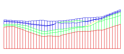
Sample cross section
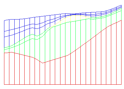
Sample cross section


Smoothing Tolerance
When the Solids → MODFLOW command is executed with the Boundary Matching option, it is common to have seams that occupy only a portion of a layer as shown in the above cross sections. The top and bottom elevations for cells adjacent to these seams must be adjusted by GMS using a "smoothing" process to ensure that there are not drastic cell size differences in the horizontal direction from one cell to the next. The smoothing is accomplished by iteratively changing the elevation of selected cells until the cell elevations change less than the Smoothing Tolerance specified in the Solids → MODFLOW Options dialog.
Minimum Thickness
This option enables avoiding extremely thin layers at edges of pinchouts and represents the minimum thickness of grid cells created from the solids. Solids with thickness less than this amount are ignored and the surrounding material is used instead. This property is assigned in the solids Properties dialog. The figure below demonstrates the application of this property.
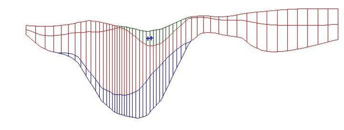
Small minimum thickness
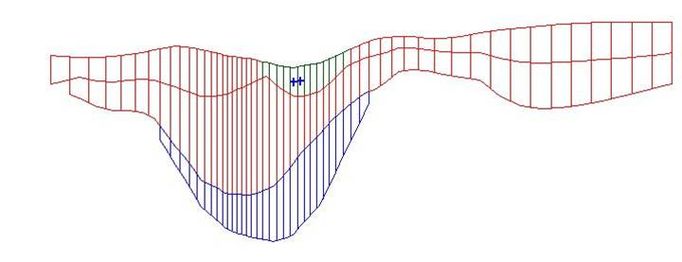
Larger minimum thickness


Top Cell Bias
The top cell bias is the percentage of the thickness which is assigned to the top layer of the MODFLOW grid create from the solids. The thickness of the top layer increases as the top cell bias increases. A large top cell bias can be used to prevent top-layer cells from going dry. This property is assigned in the solids properties dialog.
Grid Overlay
The Grid Overlay option is one of the three basic options for the Solids → MODFLOW command. The Grid Overlay option is similar to the Boundary Matching option. While the Boundary Matching option precisely matches stratigraphic boundaries, it does have some drawbacks. It can result in very thin layers at certain locations in the grid such as transition points at the boundary of a solid that pinches out to a sharp edge. In some cases, these thin layers can cause stability problems with MODFLOW or with a subsequent transport analysis. For such cases, the Grid Overlay method or the Grid Overlay with Keq method may provide superior results.
With the Grid Overlay option, no layer range assignments are necessary. Once the solids and grid are created, the Solids → MODFLOW command can be immediately selected. For each vertical column of cells, GMS intersects a vertical ray through the cell center and finds the highest and lowest intersection, i.e. the top and bottom of the entire set of solids. These elevations become the top and and bottom elevation of the entire grid. The elevations of any intermediate layer boundaries are then linearly interpolated between these two extremes. The material properties are then assigned by computing the xyz coordinates of the center of each cell and determining which solid encloses the cell center. The material properties from that solid are then assigned to the cell. The result is shown in the following figure (compare this to the example shown in the Boundary Matching topic). Note that the boundaries of the solids are not preserved as accurately as they are with the boundary matching algorithm. However, the cell sizes are much more consistent and extremely thin cells are avoided.


Minimum Thickness
In some cases, the set of solids used with the Grid Overlay method may have thin sections where the vertical thickness of the entire set of solids becomes extremely small. In such cases, the resulting grid cells become very thin as they are "squeezed" in this thin region. The cell thickness in these regions can be controlled using the Minimum Thickness value in the Solids Attributes dialog. When each vertical column of cells is processed, the height of the cells in the column is compared to the minimum thickness. If the cell height is less than the minimum, one or more cells at the bottom of the grid are inactivated until the minimum thickness is satisfied.
Grid Overlay with Keq
The Grid Overlay with K Equivalent option is one of the three basic options for the Solids → MODFLOW command. This option is very similar to the Grid Overlay option.
One of the problems with the Grid Overlay option is that if there is a relatively thin layer in the solids and the layer does not happen to encompass any cell centers or it encompasses few cell centers, the layer will be under-represented in the MODFLOW grid. This becomes particularly important if the layer is meant to represent a low permeability layer. For such cases, the Grid Overlay with K Equivalent option may give superior results. The Grid Overlay with K Equivalent method is identical to the Grid Overlay method in terms of how the elevations of the grid cells are defined. The two methods differ in how the material properties are assigned. Rather than simply assigning materials based on which solid encompasses the cell centers, the Keq method attempts to compute a custom Kh and Kv value for each cell. When assigning the material properties to a cell, GMS computes the length of each solid in the cell (from a vertical line at the cell center that intersects the solids) and computes an equivalent Kh, Kv, and storage coefficient for the cell that takes each of the solids in the cell into account. Thus, the effect of a thin seam in a cell would be included in the Kh and Kv values for the cell.
The equivalent Kh is computed as follows:
- where Khi is the Kh of a solid and Mi is the length of the same solid intersected at the cell center.
The equivalent Kv is computed as follows:

- where Kvi is the Kv of a solid and Mi is the length of the same solid intersected at the cell center.
A horizontal cross section through a sample grid defined via the Grid Overlay with Keq method is shown below. The colors represent the resulting Kh values. Note how the K values transition at the boundaries of the solids.

Parameter Estimation
Caution should be taken when using the Grid Overlay with Keq method when performing automated parameter estimation. The "key value" approach to defining parameter zones for PEST requires that the values assigned to the zones be unique within each zone. With the Boundary Matching and Grid Overlay methods, the key values could be assigned to the solids and the values would be properly inherited by the grid cells. With the Grid Overlay with Keq method, the parameter values are "blurred" at the edges of the solids and the key values assigned to the solids would be lost.
GMS – Groundwater Modeling System | ||
|---|---|---|
| Modules: | 2D Grid • 2D Mesh • 2D Scatter Point • 3D Grid • 3D Mesh • 3D Scatter Point • Boreholes • GIS • Map • Solid • TINs • UGrids | |
| Models: | FEFLOW • FEMWATER • HydroGeoSphere • MODAEM • MODFLOW • MODPATH • mod-PATH3DU • MT3DMS • MT3D-USGS • PEST • PHT3D • RT3D • SEAM3D • SEAWAT • SEEP2D • T-PROGS • ZONEBUDGET | |
| Aquaveo | ||