|
|
| Line 137: |
Line 137: |
| *''Anis1'' | | *''Anis1'' |
| *''Anis2'' | | *''Anis2'' |
|
| |
| ==Variograms==
| |
| ===Creating Experimental Variograms===
| |
| A new experimental variogram is computed by selecting the '''New''' button under the list of experimental variograms. This button brings up the ''Experimental Variogram'' dialog.
| |
|
| |
| ====Lags====
| |
| When computing an experimental variogram, it is impractical to plot a variance for each scatter point with respect to each of the other scatter points. Therefore, distances are subdivided into a number of intervals called lags as illustrated in the following figure. The distance between each pair of scatter points is checked to see which lag interval it lies within. The variances for all pairs of points whose separation distance falls within the same lag interval are averaged. The resulting average is plotted in the experimental variogram vs. the distance corresponding to the lag interval. Therefore, there is one point in the experimental variogram plot for each lag. The lag intervals are defined in the ''Experimental Variogram'' dialog by entering a total number of lags, a unit lag separation distance, and a lag tolerance. In most cases, the lag tolerance should be one half of the unit lag separation distance; the tolerance can be smaller to allow for data on a pseudo-regular grid. A pair will be included in multiple lags if the tolerance is greater than one-half of the unit lag separation distance.
| |
|
| |
| {{hide in print|[[Image:lags.png|center|550px]]}}
| |
| {{only in print|[[Image:lags.png|center|300px]]}}
| |
|
| |
| =====Semivariogram=====
| |
|
| |
| The semivariogram is the most common type of variogram. The semivariogram value for a lag interval is computed as:
| |
|
| |
| <!--<math>\gamma (h) = \frac{1}{2N} \sum_{i=1}^N \Big( f_{1i}-f_{2i} \Big) ^2</math>-->
| |
| :[[Image:variogrameq1.jpg]]
| |
|
| |
| where ''N'' is the number of pairs of points whose separation distance falls within the lag interval and ''f<sub>1i</sub>'' and ''f<sub>2i</sub>'' are the values at the head and tail of each pair of points. The head and tail are defined as follows:
| |
|
| |
| [[Image:tailhead.png|thumb|center||250 px|Naming convention for pairs of scatter points]]
| |
|
| |
| =====Covariance=====
| |
|
| |
| The covariance is the traditional covariance used in statistics. The covariance value for a lag interval is computed as:
| |
|
| |
| <!--<math>C(h) = \frac{1}{N} \sum_{i=1}^N \Big( f_{2i}f_{1i}-m_{-h}m_{+h} \Big) </math>-->
| |
| :[[Image:variogrameq2.jpg]]
| |
|
| |
| where ''m<sub>-h</sub>'' and ''m<sub>+h</sub>'' are the mean of the head and tail values respectively.
| |
|
| |
| =====Correlogram=====
| |
|
| |
| The correlogram is computed by standardizing the covariance by the standard deviation of the head and tail values.
| |
|
| |
| <!--<math>\rho (h) = \frac{C(h)}{\sigma _{-h} \sigma _{+h}}</math>-->
| |
| :[[Image:variogrameq3.jpg]]
| |
|
| |
| where ''s<sub>-h</sub>'' and ''s<sub>+h</sub>'' are the standard deviation of the head and tail values respectively.
| |
|
| |
| =====General Relative Semivariogram=====
| |
|
| |
| This variogram is computed by standardizing the semivariogram computed using equation 9.38 by the squared mean of the data values in each lag:
| |
|
| |
| <!--<math>\gamma _{GR}(h) = \dfrac{\gamma (h)}{\left ( \dfrac{m_{-h}+m_{+h}}{2} \right ) ^2}</math>-->
| |
| :[[Image:variogrameq4.jpg]]
| |
|
| |
| =====Pairwise Relative Semivariogram=====
| |
|
| |
| With this variogram, each pair is normalized by the squared average of the tail and head values.
| |
|
| |
| <!--<math>\gamma_{PR}(h) = \frac{1}{2N} \dfrac{(f_{1i}-f_{2i})^2}{ \left [ \dfrac{(f_{1i}-f_{2i})^2}{2} \right ] ^2}</math>-->
| |
| :[[Image:variogrameq5.jpg]]
| |
|
| |
| Experience has shown that the general relative and pairwise relative semivariograms are effective in revealing spatial structure and anisotropy when the scatter points are sparse (Deutsch & Journel, 1992). Because of the divisors in equations 9.41 and 9.42, these semivariograms should only be used on positively skewed datasets.
| |
|
| |
| =====Semivariogram of Logarithms=====
| |
|
| |
| This variogram is computed by applying equation 9.38 to the natural logarithms of the data values:
| |
|
| |
| <!--<math>\gamma _L (h) = \frac{1}{2N} \sum_{i=1}^N \Big( ln(f_{1i})-ln(f_{2i}) \Big) ^2</math>-->
| |
| :[[Image:variogrameq5a.jpg]]
| |
|
| |
| =====Semirodogram=====
| |
|
| |
| The semirodogram is similar to the traditional semivariogram except that the square root of the absolute difference is used rather than the squared difference:
| |
|
| |
|
| |
| <!--<math>\gamma _R (h) = \frac{1}{2N} \sum_{i=1}^N \sqrt{\left\vert f_{1i}-f_{2i} \right\vert}</math>-->
| |
| [[Image:variogrameq6.jpg]]
| |
|
| |
|
| |
| =====Semimadogram=====
| |
|
| |
| The semimadogram is similar to the traditional semivariogram, except that the absolute difference is used rather than the squared difference:
| |
|
| |
| <!--<math>\gamma _M (h) = \frac{1}{2N} \sum_{i=1}^N \left\vert f_{1i}-f_{2i} \right\vert</math>-->
| |
| :[[Image:variogrameq7.jpg]]
| |
|
| |
| The semirodogram and the semimadogram are particularly effective for establishing range and anisotropy. They should not be used for modeling the nugget of semivariograms (Deutsch & Journel, 1992).
| |
|
| |
| =====Viewing the Experimental Variograms=====
| |
|
| |
| After setting up the lag interval and choosing a variogram type, the '''OK''' button is selected in the ''Experimental Variogram'' dialog. At this point, the experimental variogram is computed. For large scatter point sets, this may take a significant amount of time.
| |
|
| |
| Once the experimental variogram is computed, it is added to the list of experimental variograms in the upper right corner of the ''Variogram Editor'' and it is displayed in the variogram plotting window. One of the variograms in the list is always highlighted. The name, color, and symbols (used to plot the variogram) of the highlighted variogram can be edited. In addition, the display of each variogram can be turned on and off so any combination of experimental variograms can be plotted. Selecting the '''Delete''' button deletes the highlighted variogram. Selecting the '''Edit''' button causes the ''Experimental Variogram'' dialog to come up initialized with the values used in the computation of the highlighted variogram. When the '''OK''' button is selected, the values of the variogram are recomputed.
| |
|
| |
| ===Creating Model Variograms===
| |
| Once a set of experimental variograms are computed, one is chosen and a model variogram is constructed to fit the experimental variogram. The model variogram is constructed using the items in the lower half of the Variogram Editor.
| |
|
| |
| ====Model Functions====
| |
| Four types of model functions are supported for building model variograms. Each of the functions are characterized by a nugget, contribution, and range.
| |
|
| |
| [[Image:modelvar.png|thumb|center|300 px|The parameters used to define a model variogram]]
| |
|
| |
| The nugget represents a minimum variance. The contribution is sometimes called the "sill" and represents the average variance of points at such a distance away from the point in question that there is no correlation between the points. The range represents the distance at which there is no longer a correlation between the points.
| |
|
| |
| The four model functions supported are:
| |
|
| |
| =====Spherical Model=====
| |
|
| |
| The Spherical Model is defined by a range ''-a-'' and a contribution ''-c-'' as:
| |
|
| |
| <!--<math>\gamma (h) =
| |
| \begin{cases}
| |
| c \left [ 1.5 \frac{h}{a}-0.5 \left ( \frac{h}{a} \right ) ^3 \right ], & \text{if } \frac{h}{a} \le a \\
| |
| c & \text{if } \frac{h}{a} > a
| |
| \end{cases}</math>-->
| |
| :[[Image:variogrameq8.jpg]]
| |
|
| |
| =====Exponential Model=====
| |
|
| |
| The Exponential Model is defined by a parameter ''-a-'' and a contribution ''-c-'' as:
| |
|
| |
| <!--<math>\gamma (h) = c \left [ 1- \text{exp} \left ( - \frac{3h}{a} \right ) \right ]</math>-->
| |
| :[[Image:variogrameq9.jpg]]
| |
|
| |
| =====Gaussian Model=====
| |
|
| |
| The Gaussian Model defined by a parameter ''-a-'' and a contribution ''-c-'' as:
| |
|
| |
| <!--<math>\gamma (h) = c \left [ 1- \text{exp} \left ( - \frac{3h^2}{a^2} \right ) \right ]</math>-->
| |
| :[[Image:variogrameq10.jpg]]
| |
|
| |
| =====Power Model=====
| |
|
| |
| The Power Model is defined by a power ''0 < a < 2'' and a slope ''c'' as:
| |
|
| |
| <!--<math>\ \gamma (h) = ch^a</math>-->
| |
| :[[Image:variogrameq11.jpg]]
| |
|
| |
| =====Nested Structures=====
| |
|
| |
| A model variogram is constructed using a combination of one or more model functions. Each instance of a model function is called a "nested structure". A nested structure is created by selecting the '''New''' button in the ''Nested Structure'' section of the dialog. A new structure is created and added to the list of nested structures. The model variogram plotted in the variogram plot window represents the combination of all of the nested structures in the list. One of the nested structures in the list is highlighted at all times. The selected structure can be deleted by selecting the '''Delete''' button under the list. The name, model function type, contribution, and range of the selected structure can be edited (the nugget is the same for all nested structures, i.e., only the contribution and range of each structure are summed). As the parameters defining the structure are altered, the plot of the model variogram is updated dynamically in the variogram plot window. This type of instantaneous feedback provides a powerful tool for "sculpting" a model variogram in an intuitive manner until it fits the selected experimental variogram.
| |
|
| |
| In most cases, a single nested structure is adequate. For cases with complex experimental variograms, using multiple nested structures to define the model variogram can prove useful.
| |
|
| |
| ===Modeling Anisotropy===
| |
| Some datasets exhibit anisotropy, i.e., the correlation between scatter points changes with direction. For example, due to the depositional history of an alluvial soil deposit, parameters such as porosity and hydraulic conductivity may be most strongly correlated in one direction. This means the differences in the data values change relatively little in one direction compared to how much they change with distance in the orthogonal direction. The direction corresponding to the highest correlation (smallest change) is called the major principal direction and the orthogonal direction is the minor principal direction.
| |
|
| |
| One of the more powerful features of the kriging method is that anisotropy can be detected by generating experimental variograms in orthogonal directions and looking for differences. When anisotropy exists, the model variogram can be constructed to match the anisotropy and ensure that the differences in the continuity of the data each of the orthogonal directions is accurately modeled in the interpolated dataset.
| |
|
| |
| ====Detecting Anisotropy====
| |
| Anisotropy can be detected by generating a focused experimental variogram in each orthogonal direction and observing whether or not there are significant differences in the resulting variograms. When constructing an experimental variogram with the ''Experimental Variogram'' dialog, directional data corresponding to an axis of anisotropy can be entered. The meaning of the directional data is illustrated in the following figure:
| |
|
| |
| [[Image:azimuth.png|thumb|center|400 px|The directional data used to detect anisotropy]]
| |
|
| |
| When a scatter point is compared with each of the other scatter points to compute the experimental variogram, only those points falling within the shaded area shown in the figure above are considered. The shaded area is defined by the azimuth angle, the azimuth bandwidth, the half window azimuth tolerance, and the lag intervals. For isotropic conditions, the half window azimuth tolerance should be set to 90<sup>o</sup> (the default value). This forces all points to be included in the calculation of the experimental variogram.
| |
|
| |
| Anisotropy is typically detected using a trial and error process. Pairs of experimental variograms are generated, the pairs being offset from each other by an azimuth angle of 90<sup>o</sup>. If anisotropy exists, the ranges of the two variograms will differ as shown below. If the data are isotropic, the azimuth angle will have little effect on the resulting experimental variograms. The angles which produce the pair of experimental variograms with the largest difference in ranges represent the principal axes of anisotropy. The variogram with the larger range represents the major principal axis and the variogram with the shorter range represents the minor principal axis.
| |
|
| |
| [[Image:anisotropy.png|thumb|center|400 px|Experimental and model variograms for anisotropic conditions]]
| |
|
| |
| ====Anisotropy Method====
| |
| Once anisotropy has been detected, the next step is to model the anisotropy using the model variogram.
| |
|
| |
| The azimuth angle corresponding to that major principal axis (the one with the longer range) should be entered in the azimuth angle field in the lower left corner of the ''Variogram Editor'' (the dip and plunge fields are for 3D kriging and are dimmed for 2D interpolation). A model variogram should then be constructed which fits the experimental variogram corresponding to the major principal direction. The anis1 parameter in the ''Variogram Editor'' should then be changed to a value other than unity (the default value). Changing the anis1 parameter to a value less than unity causes two curves to be drawn for the model variogram as shown in the above figure. The second curve corresponds to the original curve with the range parameter multiplied by the anis1 value. In other words, the anis1 parameter represents the range in the minor direction divided by the range in the major direction. The anis1 parameter should be altered until the second curve fits the experimental variogram corresponding to the minor principal axis of anisotropy. Each of the nested structures has an anis1 parameter that can be edited. Once again, as the anis1 parameter is altered, the variogram plot is updated dynamically, allowing a fit to be made in a simple intuitive fashion. Once the correct anis1 factor is found, the ''Variogram Editor'' should be exited and the azimuth and anis1 factors should be entered in the [[GMS:Kriging Options|''Search Ellipsoid'']] dialog to define a search ellipse that matches the variogram anisotropy.
| |
|
| |
| ====Saving Variograms====
| |
| Once a variogram or set of variograms is defined, the variograms are saved with the dataset files when the project is saved to disk. Thus, when the project is read back in to GMS, the variograms are ready to be used for interpolation and do not need to be redefined.
| |
|
| |
|
| ==Related Topics== | | ==Related Topics== |
Kriging is a method of interpolation named after a South African mining engineer named D. G. Krige who developed the technique in an attempt to more accurately predict ore reserves. Over the past several decades kriging has become a fundamental tool in the field of geostatistics.
Kriging is based on the assumption that the parameter being interpolated can be treated as a regionalized variable. A regionalized variable is intermediate between a truly random variable and a completely deterministic variable in that it varies in a continuous manner from one location to the next and therefore points that are near each other have a certain degree of spatial correlation, but points that are widely separated are statistically independent (Davis, 1986). Kriging is a set of linear regression routines which minimize estimation variance from a predefined covariance model.
The kriging routines implemented in GMS are based on the Geostatistical Software Library (GSLIB) routines published by Deutsch and Journel (1992). Since kriging is a rather complex interpolation technique and includes numerous options, a complete description of kriging is beyond the scope of this reference manual. It is strongly encouraged to refer the GSLIB textbook for more information:
- Deutsch, C.V., & A.G. Journel. GSLIB: Geostatistical Software Library and User's Guide. Oxford University Press, New York, 1992.
Other good references on kriging include:
- Royle, A.G., F.L. Clausen, & P. Frederiksen. Practical Universal Kriging and Automatice Contouring. Geo-Processing, Vol. 1, No. 4, 1981.
- Davis, J.C. Statistics and Data Analysis in Geology. John Wiley & Sons, New York, 1986.
- Lam, N.S. Spatial Interpolation Methods: A Review. The American Cartographer. Vol. 10, No. 2, 1983.
- Heine, G.W., A Controlled Study of Some Two-Dimensional Interpolation Methods, COGS Computer Contributions, Vol. 2, No. 2.
- Olea, T.A., Optimal Contour Mapping using Universal Kriging. J. Geophys. Research, Vol. 79, No. 5, 1974.
- Journel, A.G., & Huijbregts, C.J. Mining Geostatistics. Academic Press, New York, NY, 1978.
Kriging Techniques
A powerful set of kriging techniques with varying degrees of sophistication have been implemented in GMS. The selection of the Kriging method and the definition of the variograms are accomplished using the Kriging Options dialog. There are several differences between 2D and 3D Kriging. The supported techniques include:
Ordinary Kriging
The first step in ordinary kriging is to construct a variogram from the scatter point set to be interpolated. A variogram consists of two parts: an experimental variogram and a model variogram. Suppose that the value to be interpolated is referred to as f. The experimental variogram is found by calculating the variance (g) of each point in the set with respect to each of the other points and plotting the variances versus distance (h) between the points. Several formulas can be used to compute the variance, but it is typically computed as one half the difference in f squared.
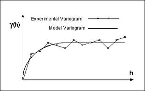
Experimental and model variogram used in Kriging
Once the experimental variogram is computed, the next step is to define a model variogram. A model variogram is a simple mathematical function that models the trend in the experimental variogram.
As can be seen in the above figure, the shape of the variogram indicates that at small separation distances, the variance in f is small. In other words, points that are close together have similar f values. After a certain level of separation, the variance in the f values becomes somewhat random and the model variogram flattens out to a value corresponding to the average variance.
Once the model variogram is constructed, it is used to compute the weights used in kriging. The basic equation used in ordinary kriging is as follows:
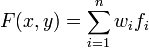
Where n is the number of scatter points in the set, fi are the values of the scatter points, and wi are weights assigned to each scatter point.
This equation is essentially the same as the equation used for inverse distance weighted interpolation (equation 9.8) except that rather than using weights based on an arbitrary function of distance, the weights used in kriging are based on the model variogram. For example, to interpolate at a point P based on the surrounding points P1, P2, and P3, the weights w1, w2, and w3 must be found. The weights are found through the solution of the simultaneous equations:


where S(dij) is the model variogram evaluated at a distance equal to the distance between points i and j. For example, S(d1p) is the model variogram evaluated at a distance equal to the separation of points P1 and P. Since it is necessary that the weights sum to unity, a fourth equation is added:
Since there are now four equations and three unknowns, a slack variable, l, is added to the equation set. The final set of equations is as follows:


The equations are then solved for the weights w1, w2, and w3. The f value of the interpolation point is then calculated as:

By using the variogram in this fashion to compute the weights, the expected estimation error is minimized in a least squares sense. For this reason, kriging is sometimes said to produce the best linear unbiased estimate. However, minimizing the expected error in a least squared sense is not always the most important criteria and in some cases, other interpolation schemes give more appropriate results (Philip & Watson, 1986).
An important feature of kriging is that the variogram can be used to calculate the expected error of estimation at each interpolation point since the estimation error is a function of the distance to surrounding scatter points. The estimation variance can be calculated as:

When interpolating to an object using the kriging method, an estimation variance dataset is always produced along with the interpolated dataset. As a result, a contour or isosurface plot of estimation variance can be generated on the target mesh or grid.
Simple Kriging
Simple kriging is similar to ordinary kriging except that the following equation is not added to the set of equations:
and the weights do not sum to unity. Simple kriging uses the average of the entire data set while ordinary kriging uses a local average (the average of the scatter points in the kriging subset for a particular interpolation point). As a result, simple kriging can be less accurate than ordinary kriging, but it generally produces a result that is "smoother" and more aesthetically pleasing.
Universal Kriging
One of the assumptions made in kriging is that the data being estimated are stationary. That is, when moving from one region to the next in the scatter point set, the average value of the scatter points is relatively constant. Whenever there is a significant spatial trend in the data values such as a sloping surface or a localized flat region, this assumption is violated. In such cases, the stationary condition can be temporarily imposed on the data by use of a drift term. The drift is a simple polynomial function that models the average value of the scatter points. The residual is the difference between the drift and the actual values of the scatter points. Since the residuals should be stationary, kriging is performed on the residuals and the interpolated residuals are added to the drift to compute the estimated values. Using a drift in this fashion is often called "universal kriging."
Kriging Options Dialog
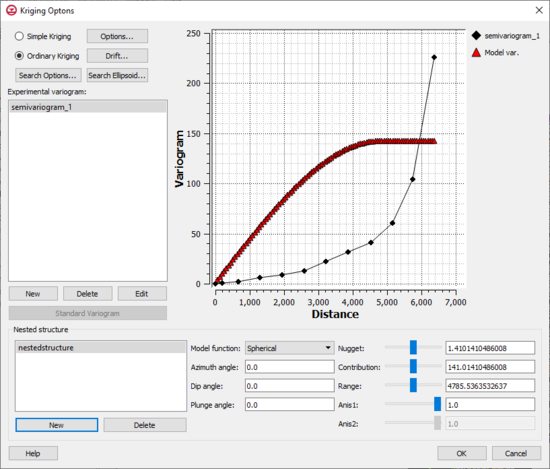
The
Kriging Options dialog
The kriging options can be edited with the Kriging Options dialog. This dialog is reached through the Interpolate UGrid to Ugrid dialog. The options in the Kriging Options dialog are as follows:
- Simple Kriging – Use the simple Kriging method.
- Ordinary Kriging – Use the ordinary Kriging method.
- Options – Opens the Interpolate – Advanced dialog with options to truncate the data and set anistropy options.
- Drift – Brings up the Drift Coefficients dialog. When performing universal kriging a drift function should be defined. Each of the toggles in the dialog represents a single component of the polynomial equation defining the drift. Initially, all of the toggles off by default. Turning on coefficients enables universal kriging and defines the drift polynomial. For example, to use a planar drift function, only the linear terms should be used.
- Search Options – Brings up the Search Options dialog. The Minimum and Maximum values in the Number of points to use for kriging controls how many of the points found in the search radius are actually used in the kriging calculations. If fewer than the minimum value are found, a default value (-999) is assigned to the interpolation point. If greater than the maximum value is found, the closest points are used.
- The input data cutoff values are used to screen out data values outside the specified range. Points with values outside this range are ignored.
- If the Octant option is selected in the search type section, a maximum of N points in each of the eight octants (for 2D a quadrant is used) surrounding the interpolation point are used in the calculations. This method results in better performance with clustered data. If the Normal method is selected, the octant approach is not used.
- Search Ellipsoid – Brings up the Search Ellipsoid dialog. When a value is interpolated to an interpolation point, only a subset of the scatter points in the vicinity of the interpolation point are used in the calculations. The items in the Search Ellipsoid dialog control the shape of a "search space" surrounding the interpolation point. Only points in this search space are considered candidates for use in the kriging calculations.
- By default, the search space is a circle (sphere in 3D) centered at the point with a radius defined by the Maximum search radius item. For problems exhibiting anisotropy, the search space can be transformed to an ellipse (ellipsoid in 3D). The anis1 factor and the azimuth angle control the shape and orientation of the ellipse. The azimuth represents the rotation of the major principal axis clockwise from the +y axis. The anis1 factor represents the ratio of the search radius along the minor principal axis relative to the search radius (the maximum radius) in the major principal direction. In most cases, the anis1 factor and the azimuth angle should match the anis factor and azimuth angle defined in the Variogram Editor.
- Experimental variogram
- New
- Delete
- Edit
- Standard Variogram
- Nested Structure – A model variogram is constructed using a combination of one or more model functions. Each instance of a model function is called a "nested structure". The model variogram plotted in the variogram plot window represents the combination of all of the nested structures in the list. One of the nested structures in the list is highlighted at all times. In most cases, a single nested structure is adequate. For cases with complex experimental variograms, using multiple nested structures to define the model variogram can prove useful.
- New – Creates a new nested structure in the list.
- Delete – Removes the seleced nested structure.
- Model function – Allows selecting on of four types of model functions: "Spherical", "Exponetial", "Gaussian", or "Power".
- Azimuth angle
- Dip angle
- Plunge angle
- Nugget – Represents a minimum variance. The contribution is sometimes called the "sill" and represents the average variance of points at such a distance away from the point in question that there is no correlation between the points. The range represents the distance at which there is no longer a correlation between the points.
- Contribution
- Range
- Anis1
- Anis2
Related Topics

